【转】latexCommand

来源：LaTeX:Commands

This page introduces various useful commands for rendering math in LaTeX, as well as instructions for building your own commands.

Contents

• 1 Subscripts and Superscripts
• 2 Math Commands
  • 2.1 Fractions
  • 2.2 Radicals
  • 2.3 Sums, Products, Limits and Logarithms
  • 2.4 Mods
  • 2.5 Combinations
  • 2.6 Trigonometric Functions
  • 2.7 Calculus
  • 2.8 Overline and Underline
• 3 LaTeX
  • 3.1 Other Functions
• 4 Matrices
• 5 Text Styles in Math Mode
• 6 How to Build Your Own Commands
• 7 See Also

Subscripts and Superscripts

Make exponents in LaTeX with ^ and subscripts with _ as shown in the examples below.

Symbol	Command	Symbol	Command
	2^2		a_i
	2^		n_
	a^{i+1}_3		x{32}
	2^		2^a_i

Notice that we can apply both a subscript and a superscript at the same time, and that we can use crimped brackets () to tell what to apply a subscript or superscript to (compare the examples on the bottom row).

Notice also that we put curly brackets around subscripts and superscripts with more than one character. You have to do so, or you'll end up with something such as , when what you really want is .

Math Commands

Here are some commonly used math commands in LaTeX.

Fractions

Symbol	Command
	\frac 12
	\frac{2}
	\frac{1+\frac{1}{x}}

Notice that with fractions with a 1-digit numerator and a 1-digit denominator, we can simply group the numerator and the denominator together as one number. However, for fractions with either a numerator or a denominator that requires more than one character, you need to surround everything in curly brackets.

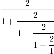
Use \cfrac for continued fractions.

Expression	Command
	\cfrac{2}{1+\cfrac{2}{1+\cfrac{2}{1+\cfrac{2}{1}}}}

Radicals

Symbol	Command
	\sqrt(2)
	\sqrt
	\sqrt
	\sqrt{x+\frac{1}{2}}
	\sqrt[3]
	\sqrt[n]

Sums, Products, Limits and Logarithms

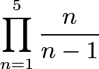
We use _ to get the 'bottom' parts of summations, products, and limits, as well as the subscripts of logarithms. We use ^ to get the 'top' parts of sums and products. (Integration symbols work the same way, as you'll see in the calculus section.) Click here for a few other commands which take 'bottom' parts.

Symbol	Command
	\sum_{i=1}^{\infty}\frac{1}
	\prod_{n=1}^5\frac{n}
	\lim_{x\to\infty}\frac{1}
	\log_n n^2

Some of these are prettier in display mode:

Symbol	Command
	\sum_{i=1}^{\infty}\frac{1}
	\prod_{n=1}^5\frac{n}
	\lim_{x\to\infty}\frac{1}

Note that we can use sums, products, and logarithms without _ or ^ modifiers.

Symbol	Command
	\sum\frac{1}
	\frac{n}
	\log n^2
	\ln e

Mods

Symbol	Command
	9\equiv 3 \bmod
	9\equiv 3 \pmod
	9\equiv 3 \mod
	9\equiv 3 \pod

Combinations

Symbol	Command
	\binom{1}
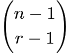
	\binom{n-1}

These often look better in display mode:

Symbol	Command
	\dbinom{9}
	\dbinom{n-1}

Trigonometric Functions

Most of these are just the abbreviation of the trigonometric function with simply a backslash added before the abbreviation.

Symbol	Command	Symbol	Command	Symbol	Command
	\cos		\sin		\tan
	\sec		\csc		\cot
	\arccos		\arcsin		\arctan
	\cosh		\sinh		\tanh
	\coth

Here are a couple examples:

Symbol	Command
	\cos^2 x +\sin^2 x = 1
	\cos 90^\circ = 0

Calculus

Below are examples of calculus rendered in LaTeX. Most of these commands have been introduced before. Notice how definite integrals are rendered (and the difference between regular math and display mode for definite integrals). The , in the integrals makes a small space before the dx.

Symbol	Command
	\frac{d}{dx}\left(x^2\right) = 2x
	\int 2x,dx = x^2+C
	\int^5_1 2x,dx = 24
	\int^5_1 2x,dx = 24
	\frac{\partial^2U}{\partial x^2} + \frac{\partial^2U}
	\frac{1}{4\pi}\oint_\Sigma\frac{1}{r}\frac{\partial U}{\partial n} ds

Overline and Underline

Symbol	Command
	\overline
	\underline

LaTeX

Other Functions

Symbol	Command	Symbol	Command	Symbol	Command
	\arg		\deg		\det
	\dim		\exp		\gcd
	\hom		\inf		\ker
	\lg		\liminf		\limsup
	\max		\min		\Pr
	\sup

Some of these functions take 'bottom' parts just like sums and limits. Some render differently in display mode and regular math mode.

Symbol	Command	Symbol	Command	Symbol	Command
	\dim_x		\gcd_x		\inf_x
	\liminf_x		\limsup_x		\max_x
	\min_x		\Pr_x		\sup_x

Matrices

We can build an array or matrix with the \begin{array} command, and use \left and \right to properly size the delimiters around the matrix:

The characteristic polynomial $f(\lambda)$ of the
$3 \times 3$ matrix
\[
\left(
\begin{array}{ccc}
a & b & c <br />d & e & f <br />g & h & i \end{array}
\right)\]
is given by the equation
\[ f(\lambda)
= \left|
\begin{array}{ccc}
\lambda - a & -b & -c <br />-d & \lambda - e & -f <br />-g & -h & \lambda - i \end{array}
\right|.\]

More simply, we can use the shortcut commands in the amsmath package:

The characteristic polynomial $f(\lambda)$ of the
$3 \times 3$ matrix
\[
\begin{pmatrix}
a & b & c <br />d & e & f <br />g & h & i
\end{pmatrix} \]
is given by the equation
\[ f(\lambda)
= \begin{vmatrix}
\lambda - a & -b & -c <br />-d & \lambda - e & -f <br />-g & -h & \lambda - i
\end{vmatrix}.\]

You can read more about how the array command works here (it works the same as tabular).

We can also use this environment to typeset any mathematics that calls for multiple columns, such as funky function definitions like this one:

\[ f(x) = \left\{ \begin{array}{ll}
x+7 & \mbox{if $5< x$};<br />x^2-3 & \mbox{if $-3 \le x \le 5$};<br />-x & \mbox{if $x < -3$}.\end{array} \right. \]

But it would be better to use the cases environment and \text command that the amsmath package provides:

\[ 
f(x) = \begin{cases}
x+7 & \text{if $5< x$}; <br />x^2-3 & \text{if $-3 \le x \le 5$};<br />-x & \text{if $x < -3$}.
\end{cases}
\]

Text Styles in Math Mode

You can render letters in various styles in math mode. Below are examples; you should be able to use these with any letters. The \mathbb requires the amsfonts package to be included in your document's preamble. Do not try to do \mathbb{year}. You'll get , and that looks nothing like it!

Symbol	Command	Symbol	Command	Symbol	Command	Symbol	Command
	\mathbb		\mathbf		\mathcal		\mathfrak
	\mathbb		\mathbf		\mathcal		\mathfrak
	\mathbb		\mathbf		\mathcal		\mathfrak

If you're persistent, you can dig a few more out of this document.

If you want to drop a little bit of text in the middle of math mode, you can use the \text command. The \text command is most useful in $$...$$ or $...$ mode, where breaking up the math mode would force the output on to a new line entirely. So

$$n^2 + 5 = 30\text{ so we have }n=\pm5$$

gives

How to Build Your Own Commands

The command \newcommand is used to create your own commands. We'll start with an example:

\documentclass[11pt]{article}
\usepackage{amsmath}

\pdfpagewidth 8.5in
\pdfpageheight 11in
\newcommand{\reci}[1]{\frac{1}{#1}}
\newcommand{\hypot}[2]{\sqrt{#1^2+#2^2}}
\newcommand{\cbrt}[1]{\sqrt[3]{#1}}

\begin{document}

The reciprocal of 2 is $\reci{2}$.

The hypotenuse has length $\hypot{3}{4}$.

I'm sick of writing `$\backslash$sqrt[3]{2}$' all the time, just to get $\cbrt{2}$.

\end{document}

The \newcommand declarations are in the preamble. Each is of the form

\newcommand{name of new command}[number of arguments]{definition}

The name of the new command, which must begin with a , is the name you'll use in the document to use the command. The number of arguments is how many inputs will be sent to the command. The definition is just normal LaTeX code, with #1, #2, #3, etc., placed where you want the inputs to go when the new command is called.

New commands can be used for all sorts of purposes, not just for making math commands you'll use a lot easier to call. For example, try this:

\documentclass[11pt]{article}
\usepackage{amsmath}

\pdfpagewidth 8.5in
\pdfpageheight 11in
\newcounter{prob_num}
\setcounter{prob_num}{1}
\newcommand{\prob}[5]{\bigskip \bigskip\arabic{prob_num}.\stepcounter{prob_num} #1
\par\nopagebreak[4]\medskip A.\ #2\hfill B.\ #3\hfill
C.\ #4\hfill D.\ #5\hfill E.\ NOTA}

\begin{document}

\prob{What is $2+2$?}{4}{5}{6}{7}

\prob{What is $\sqrt{100}$?}{81}{10}{9}{1}

\prob{Evaluate $\sum_{n=1}^\infty \frac{1}{n^2}$.}
{$\frac{1}{e}$} {$\frac{2}{\pi}$}
{$\frac{\pi^3}{8}$} {$\frac{\pi^2}{6}$}

\end{document}

In the example above, we create a new command called \prob. Each time we call \prob, we supply 5 arguments, one for the question and one for each of the multiple choices.

In the preamble and the definition of \prob, you'll see a few new LaTeX commands:

\newcounter{prob_num} creates a counter variable called prob_num

\setcounter{prob_num}{1} setsprob_num to equal 1.

In the definition of \prob, the \bigskip and \medskip commands create vertical space.

\arabic{prob_num} prints out the current value of the counter prob_num as an arabic numeral.

\stepcounter{prob_num} increments the counter prob_num by 1.

\nopagebreak[4] tells LaTeX not to break the page between the problem and the choices unless it really, really, really has to.

The \hfill commands put roughly equal space between the choices.

Once you build a body of custom commands that you will be using in many LaTeX documents, you should learn about creating your own package so you don't have to copy all your custom commands from document to document.

See Also

• Next: Packages
• Previous: Symbols