
0、History
The distribution was first introduced by Siméon Denis Poisson (1781–1840) and published, together with his probability theory, in 1837 in his work "Research on the Probability of Judgments in Criminal and Civil Matters".The work theorized about the number of wrongful convictions in a given country by focusing on certain random variables N that count, among other things, the number of discrete occurrences (sometimes called "events" or "arrivals") that take place during a time-interval of given length. The result had been given previously by Abraham de Moivre . This makes it an example of Stigler's law and it has prompted some authors to argue that the Poisson distribution should bear the name of de Moivre.
A practical application of this distribution was made by Ladislaus Bortkiewicz in 1898 when he was given the task of investigating the number of soldiers in the Prussian army killed accidentally by horse kicks; this experiment introduced the Poisson distribution to the field of reliability engineering.泊松分布由法国数学家西莫恩·德尼·泊松(Siméon-Denis Poisson)在1838年时发表,是概率论中常用的一种离散型概率分布。如果你想知道某个时间范围内,发生某件事情x次的概率是多大。这时候就可以用泊松分布轻松搞定。比如一天内中奖的次数,一个月内某机器损坏的次数等。若随机变量 X 只取非负整数值,取k值的概率为
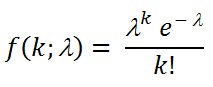
(k=0,1,2,…)
则随机变量X 的分布称为泊松分布,记作P(λ)。这个分布是泊松研究二项分布的渐近公式是时提出来的。泊松分布P (λ)中只有一个参数λ ,它既是泊松分布的均值,也是泊松分布的方差。在实际事例中,当一个随机事件,例如某电话交换台收到的呼叫、来到某公共汽车站的乘客、某放射性物质发射出的粒子、显微镜下某区域中的白血球等等,以固定的平均瞬时速率 λ(或称密度)随机且独立地出现时,那么这个事件在单位时间(面积或体积)内出现的次数或个数就近似地服从泊松分布。因此泊松分布在管理科学,运筹学以及自然科学的某些问题中都占有重要的地位。
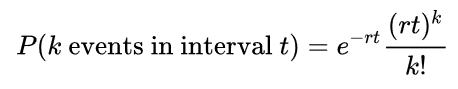
泊松分布的本质就是:已知某事件发生的频率r已知( 则λ=rt),将时间(空间等)无限分割成及其小,以使得事件成为伯努利实验,从而可以用来进行统计。
1、Basics
The Poisson distribution is popular for modelling the number of times an event occurs in an interval of time or space.
2、Assumptions: When is the Poisson distribution an appropriate model?
The Poisson distribution is an appropriate model if the following assumptions are true.
- k is the number of times an event occurs in an interval and k can take values 0, 1, 2, ….(即非负整数)
- The occurrence of one event does not affect the probability that a second event will occur. That is, events occur independently.
- The rate at which events occur is constant. The rate cannot be higher in some intervals and lower in other intervals.
- Two events cannot occur at exactly the same instant; instead, at each very small sub-interval exactly one event either occurs or does not occur.
- Or
- The actual probability distribution is given by a binomial distribution and the number of trials is sufficiently bigger than the number of successes one is asking about (see Related distributions).
If these conditions are true, then k is a Poisson random variable, and the distribution of k is a Poisson distribution.
3、Probability of events for a Poisson distribution
An event can occur 0, 1, 2, … times in an interval. The average number of events in an interval is designated
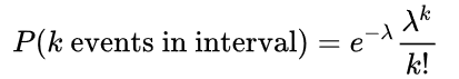
 (lambda). Lambda is the event rate, also called the rate parameter. The probability of observing
where
- λ is the average number of events per interval
- e is the number 2.71828... (Euler's number) the base of the natural logarithms
- k takes values 0, 1, 2, …
- k! = k × (k − 1) × (k − 2) × … × 2 × 1 is the factorial of k
4、Examples of probability for Poisson distributions
Examples1:
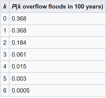
On a particular river, overflow floods occur once every 100 years on average. Calculate the probability of k = 0, 1, 2, 3, 4, 5, or 6 overflow floods in a 100-year interval, assuming the Poisson model is appropriate.
Because the average event rate is one overflow flood per 100 years, λ = 1
泊松分布的直观意义是:洪水平均100年发生一次,求洪水100年里发生k 次(0,1,2,3,4.......次)的概率分别是多少。
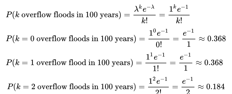


The table below gives the probability for 0 to 6 overflow floods in a 100-year period.
Examples2:
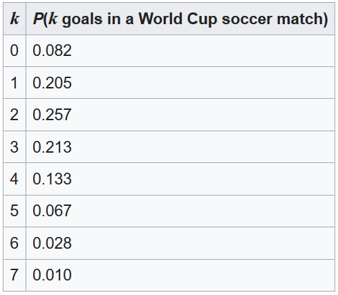
Ugarte and colleagues report that the average number of goals in a World Cup soccer match is approximately 2.5 and the Poisson model is appropriate.
Because the average event rate is 2.5 goals per match, λ = 2.5.
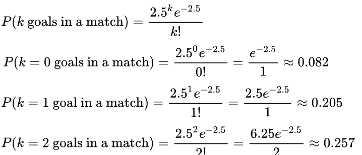
The table below gives the probability for 0 to 7 goals in a match
5、Once in an interval events: The special case of λ = 1 and k = 0
Suppose that astronomers estimate that large meteorites (above a certain size) hit the earth on average once every 100 years (λ = 1 event per 100 years), and that the number of meteorite hits follows a Poisson distribution. What is the probability of k = 0 meteorite hits in the next 100 years?

![]()
Under these assumptions, the probability that no large meteorites hit the earth in the next 100 years is roughly 0.37. The remaining 1 − 0.37 = 0.63 is the probability of 1, 2, 3, or more large meteorite hits in the next 100 years. In an example above, an overflow flood occurred once every 100 years (λ = 1). The probability of no overflow floods in 100 years was roughly 0.37, by the same calculation.
In general, if an event occurs on average once per interval (λ = 1), and the events follow a Poisson distribution, then P(0 events in next interval) = 0.37. In addition, P(exactly one event in next interval) = 0.37, as shown in the table for overflow floods.
6、Examples that violate the Poisson assumptions
The number of students who arrive at the student union per minute will likely not follow a Poisson distribution, because the rate is not constant (low rate during class time, high rate between class times) and the arrivals of individual students are not independent (students tend to come in groups).
The number of magnitude 5 earthquakes per year in a country may not follow a Poisson distribution if one large earthquake increases the probability of aftershocks of similar magnitude(非独立).
Among patients admitted to the intensive care unit of a hospital, the number of days that the patients spend in the ICU is not Poisson distributed because the number of days cannot be zero. The distribution may be modeled using a Zero-truncated Poisson distribution.
Count distributions in which the number of intervals with zero events is higher than predicted by a Poisson model may be modeled using a Zero-inflated model.
7、Occurrence
Biology example: the number of mutations on a strand of DNA per unit length.
The Poisson distribution arises in connection with Poisson processes. It applies to various phenomena of discrete properties (that is, those that may happen 0, 1, 2, 3, ... times during a given period of time or in a given area) whenever the probability of the phenomenon happening is constant in time or space. Examples of events that may be modelled as a Poisson distribution include:
- The number of mutations in a given stretch of DNA after a certain amount of radiation.
- The proportion of cells that will be infected at a given multiplicity of infection.
8、Law of rare events
 Comparison of the Poisson distribution (black lines) and the binomial distribution with n = 10 (red circles), n = 20 (blue circles), n = 1000 (green circles). All distributions have a mean of 5. The horizontal axis shows the number of events k. Notice that as n gets larger, the Poisson distribution becomes an increasingly better approximation for the binomial distribution with the same mean.
泊松分布是二项分布n很大而p很小时的一种极限形式
The rate of an event is related to the probability of an event occurring in some small subinterval (of time, space or otherwise). In the case of the Poisson distribution, one assumes that there exists a small enough subinterval for which the probability of an event occurring twice is "negligible"(n取无限大的本质). With this assumption one can derive the Poisson distribution from the Binomial one, given only the information of expected number of total events in the whole interval. Let this total number be λ,Divide the whole interval into n subintervals I1...........In of equal size, such that n > λ ,(since we are interested in only very small portions of the interval this assumption is meaningful). This means that the expected number of events in an interval Ii for each λ is equal to λ/n.Now we assume that the occurrence of an event in the whole interval can be seen as a Bernoulli trial, where the ith trial corresponds to looking whether an event happens at the subinterval Ii with probability λ/n(即泊松分布的本质是将interval分割成无限大n,即变成n个伯努利实验进行统计). The expected number of total events in n such trials would be λ. Hence for each subdivision of the interval we have approximated the occurrence of the event as a Bernoulli process of the form B(n,λ/n).. As we have noted before we want to consider only very small subintervals. Therefore, we take the limit as n goes to infinity. In this case the binomial distribution converges to what is known as the Poisson distribution by the Poisson limit theorem.
 o
oIn several of the above examples—such as, the number of mutations in a given sequence of DNA—the events being counted are actually the outcomes of discrete trials, and would more precisely be modelled using the binomial distribution, that is X~B(N,P)。In such cases n is very large and p is very small (and so the expectation np is of intermediate magnitude). Then the distribution may be approximated by the less cumbersome Poisson distribution X~Pois(ns). This approximation is sometimes known as the law of rare events, since each of the n individual Bernoulli events rarely occurs. The name may be misleading because the total count of success events in a Poisson process need not be rare if the parameter np is not small. For example, the number of telephone calls to a busy switchboard in one hour follows a Poisson distribution with the events appearing frequent to the operator, but they are rare from the point of view of the average member of the population who is very unlikely to make a call to that switchboard in that hour.
The word law is sometimes used as a synonym of probability distribution, and convergence in law means convergence in distribution. Accordingly, the Poisson distribution is sometimes called the law of small numbers because it is the probability distribution of the number of occurrences of an event that happens rarely but has very many opportunities to happen. The Law of Small Numbers is a book by Ladislaus Bortkiewicz (Bortkevitch)[37] about the Poisson distribution, published in 1898.
可以用一个比较好的帖子来详细说明(https://blog.csdn.net/ccnt_2012/article/details/81114920).大致如下:
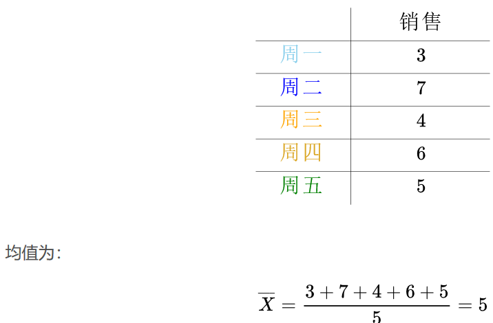
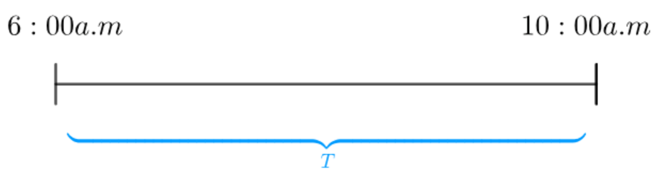
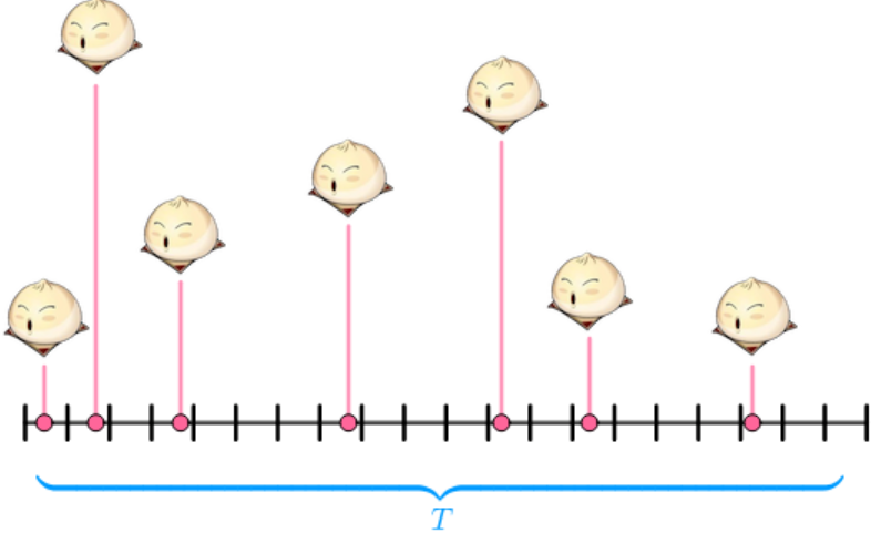
一个馒头店,早上营业8:00-10:00时间(文中的interval)。统计一周卖出的馒头(数据量小,利于理解):
interval:
以周一(λ=3)为例:
将时间段T(interval)分解成n个subinterval(注意n>λ),这里为了解释方便,将n=4。
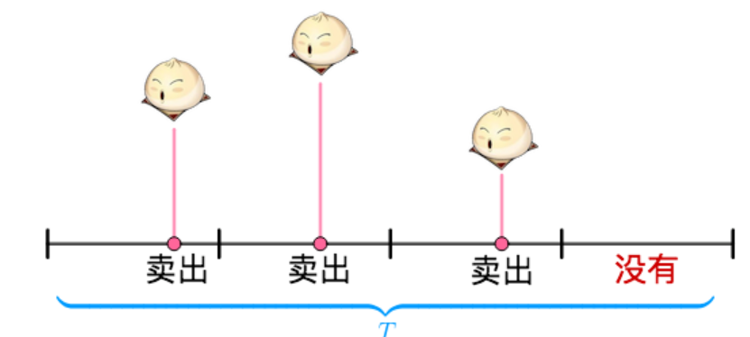
在每个时间段,可以看成伯努利实验。可以用抛硬币来类比,要不是正面(卖出),要不是反面(没有卖出)。 内卖出3个馒头的概率,就和抛了4次硬币(4个时间段),其中3次正面(卖出3个)的概率一样了。
这样的概率通过二项分布来计算就是:
![]()
以周二(λ=7)为例:
这时候还分解成4个subinterval就不合适了,因为从图中看,每个时间段,有卖出3个的,有卖出2个的,有卖出1个的,就不再是单纯的“卖出、没卖出”了。不能套用二项分布了。因为参考标题2中定义:这里每个subinterval的概率已经不是恒定的了(The rate at which events occur is constant. The rate cannot be higher in some intervals and lower in other intervals)。
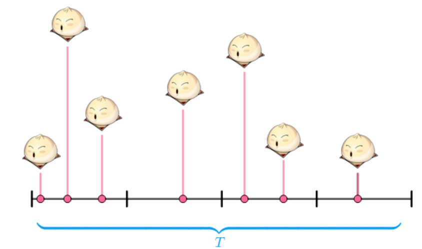
因此需要加大n,这里将n=20.
这样, 内卖出7个馒头的概率就是(相当于抛了20次硬币,出现7次正面):
周三(λ=4)、周四(λ=6)、周五(λ=5)以此类推。
抽象
将时间T分成n等分(n越大越好,取极限),卖出那么:
有了 了之后,就有:
我们来算一下这个极限:
其中:
所以:
上面就是泊松分布的概率密度函数,也就是说,在 时间内卖出
个馒头的概率为:
一般来说,我们会换一个符号,让 ,所以:
这就是泊松分布的概率密度函数。
以上相当于一步步推倒出泊松分布。其实我们可以根据标题8更加直接理解:
 subintervals
  for each
  is equal to
  . Now we assume that the occurrence of an event in the whole interval can be seen as a
  trial corresponds to looking whether an event happens at the subinterval
  . As we have noted before we want to consider only very small subintervals. Therefore, we take the limit as
 9、Poisson point process
Main article: Poisson point process
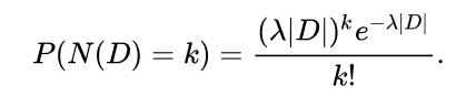
The Poisson distribution arises as the number of points of a Poisson point process located in some finite region. More specifically, if D is some region space, for example Euclidean space Rd, for which |D|, the area, volume or, more generally, the Lebesgue measure of the region is finite, and if N(D) denotes the number of points in D, then
10、Other applications in science
In a Poisson process, the number of observed occurrences fluctuates about its mean λ with a standard deviation ![]()
These fluctuations are denoted as Poisson noise or (particularly in electronics) as shot noise. See also here.
 . These fluctuations are denoted as Poisson noise or (particularly in electronics) as
 The correlation of the mean and standard deviation in counting independent discrete occurrences is useful scientifically. By monitoring how the fluctuations vary with the mean signal, one can estimate the contribution of a single occurrence, even if that contribution is too small to be detected directly. For example, the charge e on an electron can be estimated by correlating the magnitude of an electric current with its shot noise. If N electrons pass a point in a given time t on the average, the mean current is I=eN/t,since the current fluctuations should be of the order ![]() (i.e., the standard deviation of the Poisson process), the charge e can be estimated from the ratio
(i.e., the standard deviation of the Poisson process), the charge e can be estimated from the ratio ![]()
An everyday example is the graininess that appears as photographs are enlarged; the graininess is due to Poisson fluctuations in the number of reduced silver grains, not to the individual grains themselves. By correlating the graininess with the degree of enlargement, one can estimate the contribution of an individual grain (which is otherwise too small to be seen unaided).Many other molecular applications of Poisson noise have been developed, e.g., estimating the number density of receptor molecules in a cell membrane.
![]()
In Causal Set theory the discrete elements of spacetime follow a Poisson distribution in the volume.
11、Computer software for the Poisson distribution
Poisson distribution using R
The R function dpois(x, lambda) calculates the probability that there are x events in an interval, where the argument "lambda" is the average number of events per interval.
For example,
dpois(x=0, lambda=1) = 0.3678794
dpois(x=1, lambda=2.5) = 0.2052125
The following R code creates a graph of the Poisson distribution from x= 0 to 8, with lambda=2.5.
x=0:8
px = dpois(x, lambda=2.5)
plot(x, px, type="h", xlab="Number of events k", ylab="Probability of k events", ylim=c(0,0.5), pty="s", main="Poisson distribution \n Probability of events for lambda = 2.5")
 ; since the current fluctuations should be of the order
  (i.e., the standard deviation of the
  can be estimated from the ratio
  .[
.[Poisson distribution using Excel
The Excel function POISSON( x, mean, cumulative ) calculates the probability of x events where mean is lambda, the average number of events per interval. The argument cumulative specifies the cumulative distribution.
For example,
=POISSON(0, 1, FALSE) = 0.3678794
=POISSON(1, 2.5, FALSE) = 0.2052125

Poisson distribution using Python (SciPy)
The function scipy.stats.distributions.poisson.pmf(x, poissonLambda) calculates the probability that there are x events in an interval, where the argument "poissonLambda" is the average number of events per interval.


 in units of 1/time), and
  (with
(with 

 浙公网安备 33010602011771号