


深度视觉经典重读之一:卷积网络的蛮荒时代
最近在找下一篇文章的研究方向,于是重新拿起了入学前看过的一些经典老文,没想到其中蕴含的信息量这么大,原来当初naive的我根本没有领悟其中的精髓。
相对于一些琐碎的技术细节,我更关注的是【作者是怎么想出这种东西的】,或者说是【我认为有趣的点子】。
我只是出于分享和交流的目的简单地把自己的为知笔记发布了上来,所以不能保证这一系列内容适合每个人阅读。
这一篇从2012年说起,涵盖了AlexNet、Maxout、NIN、Overfeat四个经典工作。ZFNet、VGG、GoogLeNet将会在下一篇《卷积网络的工业革命》中被总结。
2012:AlexNet
2018-03-01
- 综述:
- On the test data, we achieved top-1 and top-5 error rates of 37.5% and 17.0%
- 60 million parameters and 650,000 neurons
- takes between five and six days to train on two GTX 580 3GB GPUs. (roughly 90 cycles)
- 架构:
-
Dropout. Without dropout, our network exhibits substantial overfitting. Dropout roughly doubles the number of iterations required to converge.
- ReLU。用ReLU比sigmoid或者tanh快好几倍。
- LRN. LRN的初衷是“侧面抑制”,这个表述有点意思:implements a form of lateral inhibition inspired by the type found in real neurons, creating competition for big activities amongst neuron outputs computed using different kernels. LRC reduces our top-1 and top-5 error rates by 1.4% and 1.2%, respectively.
-
Overlapping Pooling: This scheme reduces the top-1 and top-5 error rates by 0.4% and 0.3%, respectively, as compared with the non-overlapping scheme. We generally observe during training that models with overlapping pooling find it slightly more difficult to overfit.
- 预处理:
-
Given a rectangular image, we first rescaled the image such that the shorter side was of length 256, and then cropped out the central 256×256 patch from the resulting image.
-
Subtract the mean activity over the training set from each pixel.
-
(Training time)Extract random 224 × 224 patches (and their horizontal reflections) from the 256×256 images. This increases the size of our training set by a factor of 2048, though the resulting training examples are, of course, highly interdependent. Without this scheme, our network suffers from substantial overfitting, which would have forced us to use much smaller networks.
-
(Training time)PCA-based color distortion.
-
(Test time) the network makes a prediction by extracting five 224 × 224 patches (the four corner patches and the center patch) as well as their horizontalreflections (hence ten patches in all), and averaging the predictions made by the network’s softmax layer on the ten patches.
- 训练
- Initialization: We initialized the weights in each layer from a zero-mean Gaussian distribution with standard deviation 0.01. We initialized the neuron biases in the second, fourth, and fifth convolutional layers, as well as in the fully-connected hidden layers, with the constant 1. This initialization accelerates the early stages of learning by providing the ReLUs with positive inputs. We initialized the neuron biases in the remaining layers with the constant 0.
-
A batch size of 128 examples, momentum of 0.9, and weight decay of 0.0005. We found that this small amount of weight decay was important for the model to learn. Weight decay here is not merely a regularizer: it reduces the model’s training error.
![]()
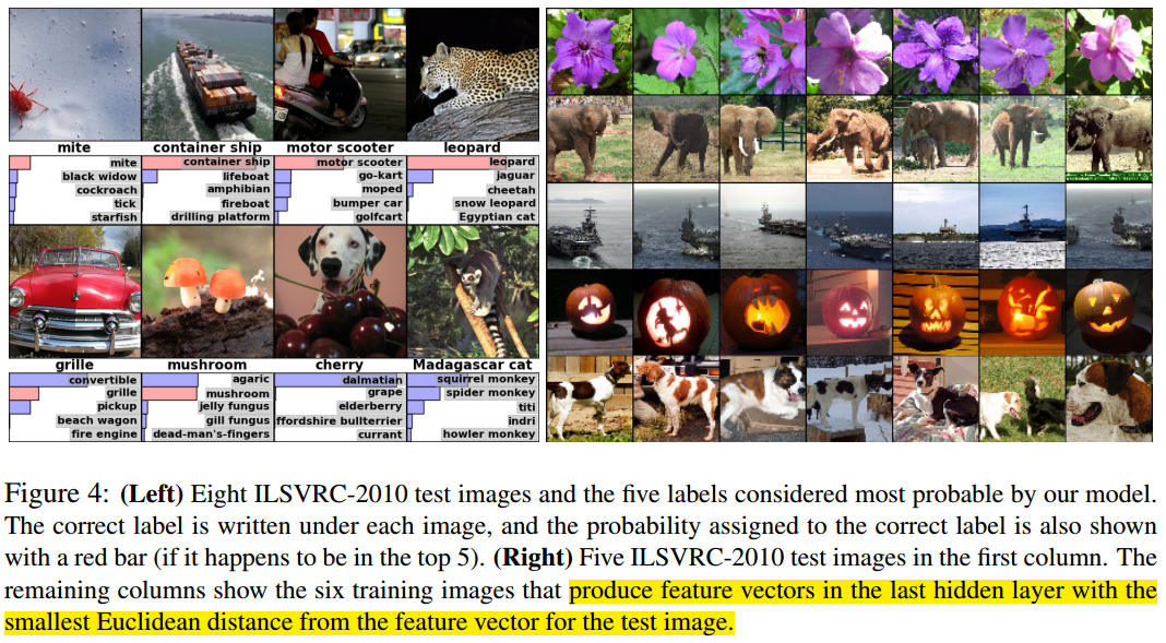
- 有效性验证:
- 拿出几张图的top-5结果,说明错的也有情可原。
- 然后找出网络所认为的相似的图片,看起来确实相似。找相似的方法就是last hidden layer产生的feature vector的欧几里得距离小。
If two images produce feature activation vectors with a small Euclidean separation, we can say that the higher levels of the neural network consider them to be similar。这样的话,也可以把网络用于image retrieval(缺点:Computing similarity by using Euclidean distance between two 4096-dimensional, real-valued vectors is inefficient, but it could be made efficient by training an auto-encoder to compress these vectors to short binary codes.)
![]()
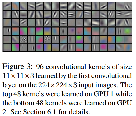
- 未解之谜,后续可以做:The kernels on GPU 1 are largely color-agnostic, while the kernels on on GPU 2 are largely color-specific. This kind of specialization occurs during every run and is independent of any particular random weight initialization (modulo a renumbering of the GPUs):
![]()

2013:Maxout
2018-03-03
本文考察了dropout作为一个提高性能的工具的内在机理。本文提出一个激活函数Maxout,它有一些好的性质,能够充分发挥dropout的作用。
We argue that rather than using dropout as a slight performance enhancement applied to arbitrary models, the best performance may be obtained by directly
designing a model that enhances dropout’s abilities as a model averaging technique.
- 由Dropout引发的思考和注意事项:
- Training using dropout differs significantly from previous approaches such as ordinary stochastic gradient descent.
- Dropout is most effective when taking relatively large steps in parameter space.
- In this regime, each update can be seen as making a significant update to a different model on a different subset of the training set.
- 与bagging的联系和启发:The ideal operating regime for dropout is when the overall training procedure resembles training an ensemble with bagging under parameter sharing constraints. This differs radically from the ideal stochastic gradient operating regime in which a single model makes steady progress via small steps.
- Another consideration is that dropout model averaging is only an approximation when applied to deep models.
- Motivation:既然上面提到only an approximation,那么怎么办能让这种approximation更好呢?Explicitly designing models to minimize this approximation error may thus enhance dropout’s performance
- 在inference time,用了dropout的层应该怎么办?
- 如果我们假设,组合不同model的softmax输出时,应该用几何平均值,那么:
- 对于只有一层且后接softmax的网络,理论上参数W应该变成W/2(输出softmax(v^T W/2+b))。
- 对于深层的情况,这不是严格成立的,但也可以这样来近似。
- Maxout本质上是一个activation function:
- 对于输入是向量的情况(FC层之后的activation):(k是超参数)
![]()
-
对于输入是feature map的情况(卷积层后的activation):a maxout feature map can be constructed by taking the maximum across k affine feature maps (i.e., pool across channels, in addition spatial locations)
- A single maxout unit can be interpreted as making a piecewise linear approximation to an arbitrary convex function. Maxout networks learn not just the relationship between hidden units, but also the activation function of each hidden unit.
-
Maxout产生的activation不是稀疏的,但是梯度是稀疏的。如果结合了dropout,dropout会使activation变成稀疏的。
-
Maxout的性质:maxout networks are universal approximators. Provided that each individual maxout unit may have arbitrarily many affine components, we show that a maxout model with just two hidden units can approximate, arbitrarily well, any continuous function of v ∈ R^n (证明见paper)
- 实验:
- MNIST。有个划分validation set和在其之上调参的技巧。既然为了避免拿test set调参的嫌疑,测定performance的时候test set只能用一次,怎么知道什么时候算是训到最好了呢?
- 前50000 train set,后10000 val set
- 根据val set上的error确定超参。取error最小的超参。记录这时候train set(50000)上的log likelihood
- 用整个60000的集合训练,直到val set(现在是训练集的子集了)上的log likelihood和之前记录的相同
- 上test set,记录结果,作为最终performance
- CIFAR-10:global contrast normalization and ZCA whitening for data augmentation. 测performance又用的另一套方法,因为最后在全集上训的时候,validation set error相对之前而言太高了(训练集扩大了,总要欠拟合一点),怎么训都没法达到之前一样:
- 确定超参之后,扔掉模型重训练
- 直到新的(训练集上的)log likelihood和之前的相同
- (再加上data augmentation的话,连上面这条都没法满足了,因为更加欠拟合了,所以只好训跟之前一样的epoch数)
- CIFAR-100:直接用CIFAR-10上调好的参数
- SVHN
- Maxout和ReLU的对比实验
- 单纯拿同样结构的网络,只是换了Maxout和ReLU的话,当然是Maxout更好
- ReLU从cross channel pooling中获益不大
- 要达到同样的performance,ReLU所需要的filter数量比Maxout多(约k倍?)
- 理论解释:section 7没仔细看,说的是不同激活函数和dropout对多模型平均的近似能力的关系,结论是折线比曲线好,maxout比ReLU好
- “ReLU+cross channel pruning”和maxout差不多。如果把后者加一个max(0,xxx),就完全等价了。实验证明,在使用dropout的情况下,这个max(0,xxx)是非常有害的。
- Dropout和普通SGD的比较:
- SGD usually works best with a small learning rate that results in a smoothly decreasing objective function, while dropout works best with a large learning rate, resulting in a constantly fluctuating objective function.
- Dropout rapidly explores many different directions and rejects the ones that worsen performance, while SGD moves slowly and steadily in the most promising direction.
- Dropout对ReLU saturation的影响:When training with SGD, we find that the rectifier units saturate at 0 less than 5% of the time. When training with dropout, we initialize the units to sature rarely but training gradually increases their saturation rate to 60%
- 在使用Dropout的情况下ReLU和Maxout的理论比较:
- In the absence of gradient through the unit, it is difficult for training to change this unit to become active again. Maxout does not suffer from this problem because gradient always flows through every maxout unit–even when a maxout unit is 0, this 0 is a function of the parameters and may be adjusted. Units that take on negative activations may be steered to become positive again later.
- 实验证明Active rectifier units become inactive at a greater rate than inactive units become active when training with dropout, but maxout units, which are always active, transition between positive and negative activations at about equal rates in each direction.
- 上一条为什么能说明maxout比ReLU好呢:We hypothesize that the high proportion of zeros and the difficulty of escaping them impairs the optimization performance of rectifiers relative to maxout
- 给maxout追加一个max(0,xxx),等效于ReLU+cross channel pruning,做实验验证上一条的假设:
- When we include a constant 0 in the max pooling, the resulting trained model fails to make use of 17.6% of the filters in the second layer and 39.2% of the filters in the second layer. A small minority of the filters usually took on the maximal value in the pool, and the rest of the time the maximal value was a constant 0.
- Maxout, on the other hand, used all but 2 of the 2400 filters in the network. Each filter in each maxout unit in the network was maximal for some training example. All filters had been utilised and tuned.
- 探究底层的梯度:
- 首先,某一层的梯度对Dropout mask的方差越大,说明dropout越有用。否则就退化成SGD了。
- We tested the hypothesis that rectifier networks suffer from diminished gradient flow to the lower layers of the network by monitoring the variance with respect to dropout masks for fixed data during training of two different MLPs on MNIST
- The variance of the gradient on the output weights was 1.4 times larger for maxout on an average training step, while the variance on the gradient of the first layer weights was 3.4 times larger for maxout than for rectifiers
- This greater variance suggests that maxout better propagates varying information downward to the lower layers and helps dropout training to better resemble bagging for the lower-layer parameters. Rectifier networks, with more of their gradient lost to saturation, presumably cause dropout training to resemble regular SGD toward the bottom of the network.

2013:Network In Network
2018-03-03
关于卷积层、抽象和线性可分的观点比较有意思
- Insight:
- 首先,指出卷积层的任务是“abstract”下层的特征,传统的filter的这种抽象层次是低的。We argue that the level of abstraction is low. By abstraction we mean that the feature is invariant to the variants of the same concept 。这种抽象是线性的,所以只适用于线性可分的特征。但是不能假设一个卷积层所要提取的特征是线性可分的,这样是不合理的。
- The conventional convolutional layer uses linear filters followed by a nonlinear activation function to scan the input.
- 冗余性来源的另一种解释:This linear convolution is sufficient for abstraction when the instances of the latent concepts are linearly separable. However, representations that achieve good abstraction are generally highly nonlinear functions of the input data. In conventional CNN, this might be compensated by utilizing an over-complete set of filters to cover all variations of the latent concepts. Namely, individual linear filters can be learned to detect different variations of a same concept.
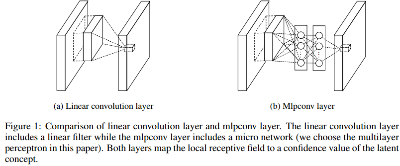
- 创新的NIN:
- 与Maxout的区别:Mlpconv layer differs from maxout layer in that the convex function approximator is replaced by a universal function approximator, which has greater capability in modeling various distributions of latent concepts.
- Instead, we build micro neural networks with more complex structures to abstract the data within the receptive field. We instantiate the micro neural network with a multilayer perceptron, which is a potent function approximator.
- 创新的GAP(insight很重要,我怎么就想不到):
- 最后的多个全连接层容易过拟合。With enhanced local modeling via the micro network, we are able to utilize global average pooling over feature maps in the classification layer, which is easier to interpret and less prone to overfitting than traditional fully connected layers.
- 把最后的feature map直接连入softmax层,就可以迫使网络generate one feature map for each correspondingcategory of the classification task in the last conv layer. One advantage of global average pooling over the fully connected layers is that it is more native to the convolution structure by enforcing correspondences between feature maps and categories. Thus the feature maps can be easily interpreted as categories confidence maps.
- 把不同空间位置上的信息加起来,是符合卷积的基本假设的(空间不变性)。Futhermore, global average pooling sums out the spatial information, thus it is more robust to spatial translations of the input.
- 再次强调:We can see global average pooling as a structural regularizer that explicitly enforces feature maps to be confidence maps of concepts (categories).
- 效果:state-of-the-art classification performances with NIN on CIFAR-10 and CIFAR-100, and reasonable performances on SVHN and MNIST datasets
![]()
- 实验
- 训练过程:batch size=128,训练集上精度停了就lr除以10.
- Dropout有用
- 对比试验证明了GAP确实减轻了过拟合,但这需要模型本身的filter的abstract能力足够强。
2013:Overfeat
2018-03-03
- The main point of this paper is to show that training a convolutional network to simultaneously classify, locate and detect objects in images can boost the classification accuracy and the detection and localization accuracy of all tasks.
- Contributions:
- The paper proposes a new integrated approach to object detection, recognition, and localization with a single ConvNet.
- We also introduce a novel method for localization and detection by accumulating predicted bounding boxes.
- We suggest that by combining many localization predictions, detection can be performed without training on background samples and that it is possible to avoid the time-consuming and complicated bootstrapping training passes. Not training on background also lets the network focus solely on positive classes for higher accuracy.
- 问题背景:
- 在ImageNet分类任务中,目标物体的尺寸和位置是多变的。所以,
- 第一种解决方案是:用sliding window的形式,以不同的scale,在图片上用卷积网络feed多次。如果这样做的话,假想一个sliding window包括了目标物体的足够identifiable的一部分,例如一个狗头,那么分类结果(一只狗)是好的,但是localizaiton和detection的结果是不好的(只框出了一个狗头)
- 第二种解决方案是:对每个sliding window,不止产生分类结果(每个类别的概率),也要产生localization和bounding box的大小(相对于这个sliding window)
- 第三种解决方案是: accumulate the evidence for each category at each location and size
- In this paper, we explore three computer vision tasks in increasing order of difficulty: (i) classification, (ii) localization, and (iii) detection. Each task is a sub-task of the next.
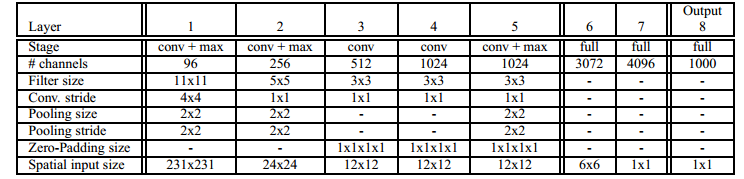
- 网络架构:
- 不用LRN
- non-overlapping pooling
- 第一第二层stride变小,feature map尺寸变大。因为本文认为A larger stride is beneficial for speed but will hurt accuracy。
- 设计了两款模型:fast和accurate。accurate的多了一层,第一个fc层的neuron变多了。刷榜的时候用了5个模型的组合。下面是fast版本。
![]()
- 类似于FCN的思路:during training, we treat this architecture as non-spatial (output maps of size 1x1), as opposed to the inference step, which produces spatial outputs. The spatial size of the feature maps depends on the input image size, which varies during our inference step. Here we show training spatial sizes. The fully-connected layers can also be seen as 1x1 convolutions in a spatial setting
- Classification
- 训练细节:
- Each image is downsampled so that the smallest dimension is 256 pixels. We then extract 5 random crops (and their horizontal flips) of size 221x221 pixels and present these to the network in mini-batches of size 128.
- momentum term of 0.6 and an L2 weight decay of 1 × 10⁻⁵.
- The learning rate is initially 5 × 10⁻² and is successively decreased by a factor of 0.5 after (30, 50, 60, 70, 80) epochs
- DropOut with a rate of 0.5 is employed on the fully connected layers (6th and 7th) in the classifier
- 技巧:Multi-scale
- The result of convolving a ConvNet on an image of arbitrary size is a spatial map of C-dimensional vectors at each scale
- 之前的工作是10-view(四角,中心,水平翻转),单一scale
- we explore the entire image by densely running the network at each location and at multiple scales.
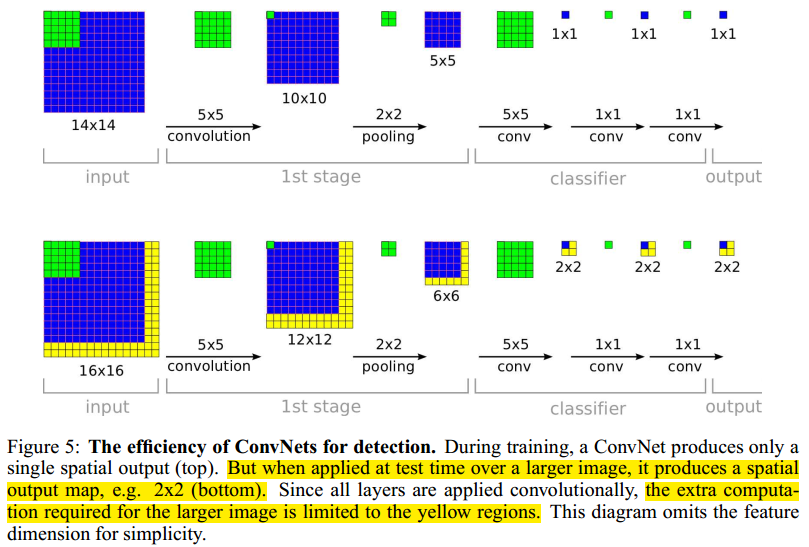
- 那怎么提高效率呢?(越看越像FCN)ConvNets are inherently efficient when applied in a sliding fashion because they naturally share computations common to overlapping regions.如下图
-
![]()
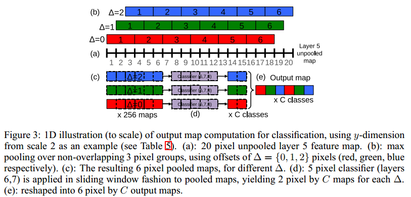
- the total subsampling ratio in the network described above is 2x3x2x3, or 36. Hence when applied densely, this architecture can only produce a classification vector every 36 pixels in the input dimension along each axis. 这样是不够好的,因为36个像素太多了,图片中真正的object可能align不到这些window 上去,所以就要降低subsampling ratio。而简单地去掉max pool的话又不太好,所以本文用了另一种比较新颖的方法,也就是所谓的resolution augmentation。这种方法可以概括为带offset的3x3 pooling,然后把不同offset(x轴方向0,1,2,y轴方向0,1,2,所以共9种offset组合)产生的pooled feature map全部经过classifier(3个fc层),把结果组合到一起,这样(最终的)subsampling ratio就没有变化:
-
![]()
- These operations can be viewed as shifting the classifier’s viewing window by 1 pixel through pooling layers without subsampling and using skip-kernels in the following layer (where values in the neighborhood are non-adjacent). Or equivalently, as applying the final pooling layer and fullyconnected stack at every possible offset, and assembling the results by interleaving the outputs.
- The procedure above is repeated for the horizontally flipped version of each image. We then produce the final classification by (i) taking the spatial max for each class, at each scale and flip; (ii) averaging the resulting C-dimensional vectors from different scales and flips and (iii) taking the top-1 or top-5 elements (depending on the evaluation criterion) from the mean class vector.
- 为什么要这样做:The exhaustive pooling scheme ensures that we can obtain fine alignment between the classifier and the representation of the object in the feature map.
- Localization:
- 从上面Classification的模型接着干:we replace the classifier layers by a regression network and train it to predict object bounding boxes at each spatial location and scale. We then combine the regression predictions together, along with the classification results at each location
- To generate object bounding box predictions, we simultaneously run the classifier and regressor networks across all locations and scales. Since these share the same feature extraction layers, only the final regression layers need to be recomputed after computing the classification network. The output of the final softmax layer for a class c at each location provides a score of confidence that an object of class c is present (though not necessarily fully contained) in the corresponding field of view. Thus we can assign a confidence to each bounding box.
- Regressor: The regression network takes as input the pooled feature maps from layer 5. It has 2 fully-connected hidden layers of size 4096 and 1024 channels, respectively. The final output layer has 4 units which specify the coordinates for the bounding box edges.
- Bounding-box merging instead of NMS. 作者认为our approach is naturally more robust to false positives coming from the pure-classification model than traditional non-maximum suppression, by rewarding bounding box coherence.
- 重要经验和以后可能的发展方向:Using a different top layer for each class in the regressor network for each class (Per-Class Regressor (PCR) in Fig. 9) surprisingly did not outperform using only a single network shared among all classes (44.1% vs. 31.3%). This may be because there are relatively few examples per class annotated with bounding boxes in the training set, while the network has 1000 times more top-layer parameters, resulting in insufficient training. It is possible this approach may be improved by sharing parameters only among similar classes (e.g. training one network for all classes of dogs, another for vehicles, etc.).
- Detection:
- 和Localization的不同点:The main difference with the localization task, is the necessity to predict a background class when no object is present
- 通常的训练方法: Traditionally, negative examples are initially taken at random for training. Then the most offending negative errors are added to the training set in bootstrapping passes.
- 这样的缺点是:
- Independent bootstrapping passes render training complicated and risk potential mismatches between the negative examples collection and training times.
- the size of bootstrapping passes needs to be tuned to make sure training does not overfit on a small set.
- 我们的创新在于:To circumvent all these problems, we perform negative training on the fly, by selecting a few interesting negative examples per image such as random ones or most offending ones. This approach is more computationally expensive, but renders the procedure much simpler
- Localization和Detection可能的改进方向:We are using L2 loss, rather than directly optimizing the intersection-over-union (IOU) criterion on which performance is measured. Swapping the loss to this should be possible since IOU is still differentiable, provided there is some overlap. (iii) Alternate parameterizations of the bounding box may help to decorrelate the outputs, which will aid network training.
<wiz_tmp_tag id="wiz-table-range-border" contenteditable="false" style="display: none;">

 浙公网安备 33010602011771号