Python数据科学手册(2) NumPy入门
NumPy(Numerical Python 的简称)提供了高效存储和操作密集数据缓存的接口。在某些方面,NumPy 数组与 Python 内置的列表类型非常相似。但是随着数组在维度上变大,NumPy 数组提供了更加高效的存储和数据操作。
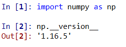
版本检查:(遵循传统,使用np作为别名导入NumPy)
2.1 理解Python中的数据类型
2.1.1 Python整形不仅仅是一个整形
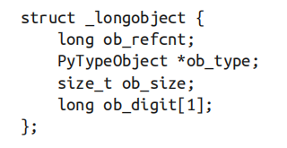
Python 3.x 中的一个整型实际上包括 4 个部分。
- ob_refcnt 是一个引用计数,它帮助 Python 默默地处理内存的分配和回收。
- ob_type 将变量的类型编码。
- ob_size 指定接下来的数据成员的大小。
- ob_digit 包含我们希望 Python 变量表示的实际整型值。
2.1.2 Python列表不仅仅是一个列表
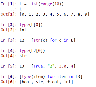
由于 Python 的动态类型特性,可以创建异构的列表。
但如果列表中的所有变量都是同一类型的,那么很多信息都会显得多余——将数据存储在固定类型的数组中会更加高效。
2.1.3 Python中的固定类型数组
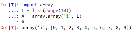
'i' 是一个数据类型码,表示数据为整型。
2.1.4 从Python列表创建数组
NumPy 要求数组必须包含同一类型的数据。如果类型不匹配,NumPy 将会向上转换(如果可行)。
如果希望明确设置数组的数据类型,可以用 dtype 关键字。
不同于 Python 列表,NumPy 数组可以被指定为多维的。

2.1.5 从头创建数组
- zeros:创建0值数组;
- ones:创建1值数组;
- arange:等差数组。
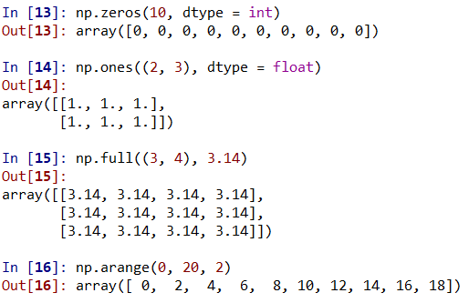
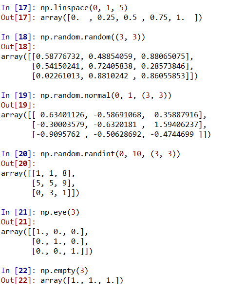
- linspace:等间隔数组;
- random.random:0~1均匀分布;
- random.normal:正态分布;
- random.randint:随机整数数组(前闭后开,例如下例中整数范围是[0, 10));
- eye:单位矩阵;
- empty:未初始化数组。
2.1.6 NumPy标准数据类型
| bool_ | Boolean (True or False) stored as a byte |
| int_ | Default integer type (same as C long; normally either int64 or int32) |
| intc | Identical to C int (normally int32 or int64) |
| intp | Integer used for indexing (same as C ssize_t; normally either int32 or int64) |
| int8 | Byte (-128 to 127) |
| int16 | Integer (-32768 to 32767) |
| int32 | Integer (-2147483648 to 2147483647) |
| int64 | Integer (-9223372036854775808 to 9223372036854775807) |
| uint8 | Unsigned integer (0 to 255) |
| uint16 | Unsigned integer (0 to 65535) |
| uint32 | Unsigned integer (0 to 4294967295) |
| uint64 | Unsigned integer (0 to 18446744073709551615) |
| float_ | Shorthand for float64. |
| float16 | Half precision float: sign bit, 5 bits exponent, 10 bits mantissa |
| float32 | Single precision float: sign bit, 8 bits exponent, 23 bits mantissa |
| float64 | Double precision float: sign bit, 11 bits exponent, 52 bits mantissa |
| complex_ | Shorthand for complex128. |
| complex64 | Complex number, represented by two 32-bit floats |
| complex128 | Complex number, represented by two 64-bit floats |
2.2 Numpy数组基础
2.2.1 Numpy数组的属性
- nidm:数组的维度;
- shape:数组每个维度的大小;
- size:数组的总大小;
- dtype:数组的数据类型;
- itemsize:数组每个元素的字节大小;
- nbytes:数组总字节大小(=itemsize*size)。

2.2.2 数组索引:获取单个元素

数组索引下标从0开始!为了获取数组的末尾索引,可以用负值索引。
2.2.3 数组切片:获取子数组
- x[start:stop:step]:如果以上 3 个参数未指定,那么它们会被分别设置默认值 start=0、stop= 维度的大小(size of dimension)和 step=1。
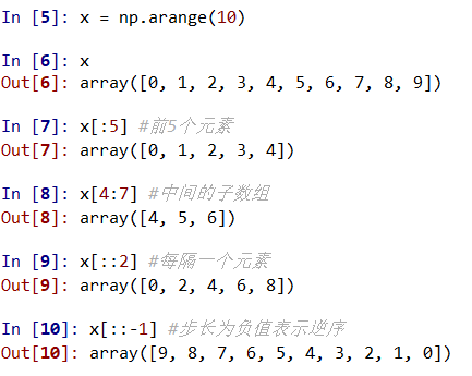
用一个冒号(:)表示空切片。

关于数组切片有一点很重要也非常有用,那就是数组切片返回的是数组数据的视图,而不是数值数据的副本。这一点也是 NumPy 数组切片和 Python 列表切片的不同之处:在 Python 列表中,切片是值的副本。

使用copy()方法,可以实现复制功能。
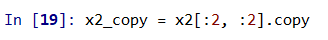
此时修改子数组,原始的数组将不会被改变。
2.2.4 数组的变形
reshape()方法返回原始数组的一个非副本视图。
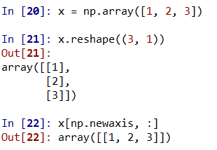
- 通过x[np.newaxis, :]获得行向量;
- 通过x[:, np.newaxis]获得列向量。
2.2.5 数组拼接和分裂
- np.concatenate():拼接或连接数组;

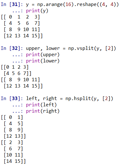
- np.vstack():垂直栈(列数不变,行数累加);
- np.hstack():水平栈(行数不变,列数累加);
- np.dstack:沿着第三个维度拼接数组。

- np.split:分裂数组;
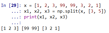
注意,N 分裂点会得到 N + 1 个子数组。
- np.hsplit:水平分裂数组;
- np.vsplit:垂直分裂数组。
2.3 NumPy数组的计算:通用函数
2.3.1 缓慢的循环
import numpy as np
np.random.seed(0)
def compute_reciprocals(values):
    output = np.empty(len(values))
    for i in range(len(values)):
        output[i] = 1.0 / values[i]
    return output
values = np.random.randint(1, 10, size=5)
print(compute_reciprocals(values))
[0.16666667 1. 0.25 0.25 0.125 ]
big_array = np.random.randint(1, 100, size=1000000)
%timeit compute_reciprocals(big_array)
1.95 s ± 18 ms per loop (mean ± std. dev. of 7 runs, 1 loop each)
运算处理的瓶颈并不是运算本身,而是 CPython 在每次循环时必须做数据类型的检查和函数的调度。每次进行倒数运算时,Python 首先检查对象的类型,并且动态查找可以使用该数据类型的正确函数。
2.3.2 通用函数介绍
NumPy 为很多类型的操作提供了非常方便的、静态类型的、可编译程序的接口,也被称作向量操作。
%timeit 1.0 / big_array
4.12 ms ± 29.8 µs per loop (mean ± std. dev. of 7 runs, 100 loops each)
NumPy 中的向量操作是通过通用函数实现的,可以看到它的完成时间比 Python 循环花费的时间更短。
np.arange(5) / np.arange(1, 6)
array([0. , 0.5 , 0.66666667, 0.75 , 0.8 ])
x = np.arange(9).reshape((3, 3))
2 ** x
array([[ 1, 2, 4],
[ 8, 16, 32],
[ 64, 128, 256]], dtype=int32)
2.3.3 探索NumPy的通用函数
1. 数组的运算
x = np.arange(4)
print("x =", x)
print("x + 5 =", x + 5)
print("x - 5 =", x - 5)
print("x * 2 =", x * 2)
print("x / 2 =", x / 2)
print("x // 2 =", x // 2) #地板除法运算
print("-x = ", -x)
print("x ** 2 = ", x ** 2)
print("x % 2 = ", x % 2)
x = [0 1 2 3]
x + 5 = [5 6 7 8]
x - 5 = [-5 -4 -3 -2]
x * 2 = [0 2 4 6]
x / 2 = [0. 0.5 1. 1.5]
x // 2 = [0 0 1 1]
-x = [ 0 -1 -2 -3]
x ** 2 = [0 1 4 9]
x % 2 = [0 1 0 1]
| Operator | Equivalent ufunc | Description |
| + | np.add | Addition (e.g., 1 + 1 = 2) |
| - | np.subtract | Subtraction (e.g., 3 - 2 = 1) |
| - | np.negative | Unary negation (e.g., -2) |
| * | np.multiply | Multiplication (e.g., 2 * 3 = 6) |
| / | np.divide | Division (e.g., 3 / 2 = 1.5) |
| // | np.floor_divide | Floor division (e.g., 3 // 2 = 1) |
| ** | np.power | Exponentiation (e.g., 2 ** 3 = 8) |
| % | np.mod | Modulus/remainder (e.g., 9 % 4 = 1) |
2. 绝对值
x = np.array([-2, -1, 0, 1, 2])
print(abs(x))
x = np.array([3 - 4j, 4 - 3j, 2 + 0j, 0 + 1j])
print(np.abs(x))
[2 1 0 1 2]
[5. 5. 2. 1.]
3. 三角函数
theta = np.linspace(0, np.pi, 4)
print("theta = ", theta)
print("sin(theta) = ", np.sin(theta))
print("cos(theta) = ", np.cos(theta))
print("tan(theta) = ", np.tan(theta))

x = [-1, 0, 1]
print("x = ", x)
print("arcsin(x) = ", np.arcsin(x))
print("arccos(x) = ", np.arccos(x))
print("arctan(x) = ", np.arctan(x))
theta = [0. 1.04719755 2.0943951 3.14159265]
sin(theta) = [0.00000000e+00 8.66025404e-01 8.66025404e-01 1.22464680e-16]
cos(theta) = [ 1. 0.5 -0.5 -1. ]
tan(theta) = [ 0.00000000e+00 1.73205081e+00 -1.73205081e+00 -1.22464680e-16]
x = [-1, 0, 1]
arcsin(x) = [-1.57079633 0. 1.57079633]
arccos(x) = [3.14159265 1.57079633 0. ]
arctan(x) = [-0.78539816 0. 0.78539816]
4. 指数和对数
x = [1, 2, 3]
print("x =", x)
print("e^x =", np.exp(x))
print("2^x =", np.exp2(x))
print("3^x =", np.power(3, x))

x = [1, 2, 4, 10]
print("x =", x)
print("ln(x) =", np.log(x))
print("log2(x) =", np.log2(x))
print("log10(x) =", np.log10(x))

x = [0, 0.001, 0.01, 0.1]
print("exp(x) - 1 =", np.expm1(x))
print("log(1 + x) =", np.log1p(x))
x = [1, 2, 3]
e^x = [ 2.71828183 7.3890561 20.08553692]
2^x = [2. 4. 8.]
3^x = [ 3 9 27]
x = [1, 2, 4, 10]
ln(x) = [0. 0.69314718 1.38629436 2.30258509]
log2(x) = [0. 1. 2. 3.32192809]
log10(x) = [0. 0.30103 0.60205999 1. ]
exp(x) - 1 = [0. 0.0010005 0.01005017 0.10517092]
log(1 + x) = [0. 0.0009995 0.00995033 0.09531018]
2.3.4 高级的通用函数特性
1. 指定输出
所有的通用函数都可以通过 out 参数来指定计算结果的存放位置。
x = np.arange(5)
y = np.empty(5)
np.multiply(x, 10, out=y)
print(y)

z = np.zeros(10)
np.power(2, x, out=z[::2])
print(z)
[ 0. 10. 20. 30. 40.]
[ 1. 0. 2. 0. 4. 0. 8. 0. 16. 0.]
2. 聚合
- reduce:对数组中各元素执行某方法;
- accumulate:保留中间过程。
x = np.arange(1, 6)
print(np.add.reduce(x))
print(np.multiply.reduce(x))
print(np.add.accumulate(x))
print(np.multiply.accumulate(x))
15
120
[ 1 3 6 10 15]
[ 1 2 6 24 120]
3. 外积
任何通用函数都可以用 outer 方法获得两个不同输入数组所有元素对的函数运算结果。
x = np.arange(1, 6)
print(np.multiply.outer(x, x))
[[ 1 2 3 4 5]
[ 2 4 6 8 10]
[ 3 6 9 12 15]
[ 4 8 12 16 20]
[ 5 10 15 20 25]]
2.4 聚合:最小值、最大值和其他值
2.4.1 数组值求和
L = np.random.random(100)
print(sum(L))
print(np.sum(L))
51.67601813148535
51.676018131485364
Python 本身可用内置的 sum 函数和 NumPy 的 sum 函数均可,但是,因为 NumPy 的 sum 函数在编译码中执行操作,所以 NumPy 的操作计算得更快一些。
big_array = np.random.rand(1000000)
%timeit sum(big_array)
%timeit np.sum(big_array)
97.8 ms ± 11.5 ms per loop (mean ± std. dev. of 7 runs, 10 loops each)
1.43 ms ± 246 µs per loop (mean ± std. dev. of 7 runs, 100 loops each)
2.4.2 最小值和最大值
big_array = np.random.rand(1000000)
print(np.min(big_array), np.max(big_array))
3.1894709762170237e-07 0.9999997837647492
多维度聚合时使用axis指定折叠轴。
M = np.arange(0, 12).reshape((3, 4))
print(M)
print(M.sum(axis = 0))
print(M.sum(axis = 1))
[[ 0 1 2 3]
[ 4 5 6 7]
[ 8 9 10 11]]
[12 15 18 21]
[ 6 22 38]
axis = 0表示行被折叠,axis = 1表示列被折叠。
其他聚合函数在下表中列出,另外,大多数的聚合都有对 NaN 值的安全处理策略(NaN-safe),即计算时忽略所有的缺失值。
| Function Name | NaN-safe Version | Description |
| np.sum | np.nansum | Compute sum of elements |
| np.prod | np.nanprod | Compute product of elements |
| np.mean | np.nanmean | Compute mean of elements |
| np.std | np.nanstd | Compute standard deviation |
| np.var | np.nanvar | Compute variance |
| np.min | np.nanmin | Find minimum value |
| np.max | np.nanmax | Find maximum value |
| np.argmin | np.nanargmin | Find index of minimum value |
| np.argmax | np.nanargmax | Find index of maximum value |
| np.median | np.nanmedian | Compute median of elements |
| np.percentile | np.nanpercentile | Compute rank-based statistics of elements |
| np.any | N/A | Evaluate whether any elements are true |
| np.all | N/A | Evaluate whether all elements are true |
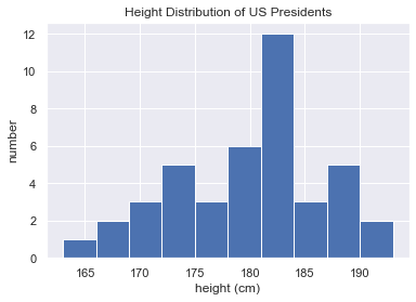
2.4.3 示例:美国总统身高
!head -4 president_heights.csv
order,name,height(cm)
1,George Washington,189
2,John Adams,170
3,Thomas Jefferson,189
import numpy as np
import pandas as pd
import matplotlib.pyplot as plt
import seaborn; seaborn.set() # 设置绘图风格

data = pd.read_csv('data/president_heights.csv')
heights = np.array(data['height(cm)'])
print(heights)

print("Mean height: ", heights.mean())
print("Standard deviation:", heights.std())
print("Minimum height: ", heights.min())
print("Maximum height: ", heights.max())

print("25th percentile: ", np.percentile(heights, 25))
print("Median: ", np.median(heights))
print("75th percentile: ", np.percentile(heights, 75))

plt.hist(heights)
plt.title('Height Distribution of US Presidents')
plt.xlabel('height (cm)')
plt.ylabel('number')
[189 170 189 163 183 171 185 168 173 183 173 173 175 178 183 193 178 173
174 183 183 168 170 178 182 180 183 178 182 188 175 179 183 193 182 183
177 185 188 188 182 185]
Mean height: 179.73809523809524
Standard deviation: 6.931843442745892
Minimum height: 163
Maximum height: 193
25th percentile: 174.25
Median: 182.0
75th percentile: 183.0
2.5 数组的计算:广播
广播可以简单理解为用于不同大小数组的二进制通用函数(加、减、乘等)的一组规则。
2.5.1 广播的介绍
a = np.array([0, 1, 2])
b = np.array([5, 5, 5])
print(a + b)

print(a + 5)
M = np.ones((3, 3))
print(M + a)

a = np.arange(3)
b = np.arange(3)[:, np.newaxis]
print(a)
print(b)
print(a + b)
[5 6 7]
[5 6 7]
[[1. 2. 3.]
[1. 2. 3.]
[1. 2. 3.]]
[0 1 2]
[[0]
[1]
[2]]
[[0 1 2]
[1 2 3]
[2 3 4]]
将一个值扩展或广播以匹配另外一个数组的形状,这里将 a 和 b 都进行了扩展来匹配一个公共的形状,最终的结果是一个二维数组。
2.5.2 广播的规则
- 规则 1:如果两个数组的维度数不相同,那么小维度数组的形状将会在最左边补 1。
- 规则 2:如果两个数组的形状在任何一个维度上都不匹配,那么数组的形状会沿着维度为 1 的维度扩展以匹配另外一个数组的形状。
- 规则 3:如果两个数组的形状在任何一个维度上都不匹配并且没有任何一个维度等于 1,那么会引发异常。
2.5.3 广播的实际应用
1. 数据的归一化
X = np.random.random((10, 3))
Xmean = X.mean(0)
Xstd = X.std(0)
print(Xmean)
print(Xstd)
X_scale = (X - Xmean) / Xstd
print(X_scale.mean(0))
print(X_scale.std(0))
[0.51706443 0.46278813 0.47832639]
[0.24168175 0.27046945 0.28595638]
[ 7.32747196e-16 -1.55431223e-16 3.10862447e-16]
[1. 1. 1.]
2. 画一个二维函数
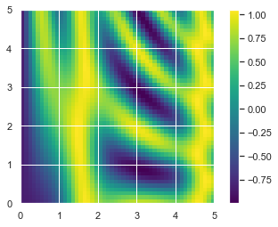
广播另外一个非常有用的地方在于,它能基于二维函数显示图像。
import numpy as np
import matplotlib.pyplot as plt

# x和y表示0~5区间50个步长的序列
x = np.linspace(0, 5, 50)
y = np.linspace(0, 5, 50)[:, np.newaxis]

z = np.sin(x) ** 10 + np.cos(10 + y * x) * np.cos(x)

plt.imshow(z, origin='lower', extent=[0, 5, 0, 5], \
           cmap='viridis')
plt.colorbar()
2.6 比较、掩码和布尔逻辑
2.6.1 示例:统计下雨天数
import numpy as np
import pandas as pd
import matplotlib.pyplot as plt

# 利用Pandas抽取降雨量,放入一个NumPy数组
rainfall = pd.read_csv('data/Seattle2014.csv')['PRCP'].values
inches = rainfall / 254 # 1/10mm -> inches
print(inches.shape)

plt.hist(inches, 40)
plt.title('2014 precipitation histogram for the city of Seattle')
(365,)

2.6.2 和通用函数类似的比较操作
| Operator | Equivalent ufunc |
| == | np.equal |
| != | np.not_equal |
| < | np.less |
| <= | np.less_equal |
| > | np.greater |
| >= | np.greater_equal |
2.6.3 操作布尔数组
1. 统计记录的个数
rng = np.random.RandomState(0)
x = rng.randint(10, size=(3, 4))
print(x)

print(np.count_nonzero(x < 6))
print(np.sum(x < 6))

# 有没有值大于8?
print(np.any(x > 8, axis=1))

# 是否所有值都小于10?
print(np.all(x < 10))
[[5 0 3 3]
[7 9 3 5]
[2 4 7 6]]
8
8
[False True False]
True
2. 布尔运算符
| Operator | Equivalent ufunc |
| & | np.bitwise_and |
| | | np.bitwise_or |
| ^ | np.bitwise_xor |
| ~ | np.bitwise_not |
print("Number days without rain: ", np.sum(inches == 0))
print("Number days with rain: ", np.sum(inches != 0))
print("Days with more than 0.5 inches:", np.sum(inches > 0.5))
print("Rainy days with < 0.1 inches :", np.sum((inches > 0) & \
(inches < 0.2)))
Number days without rain: 215
Number days with rain: 150
Days with more than 0.5 inches: 37
Rainy days with < 0.1 inches : 75
2.6.4 将布尔数组作为掩码
print(x)
print(x[x < 5])
[[5 0 3 3]
[7 9 3 5]
[2 4 7 6]]
[0 3 3 3 2 4]
注意:and 和 or 对整个对象执行单个布尔运算(逻辑),而 & 和 | 对一个对象的内容(单个比特或字节)执行多个布尔运算(按位)。对于 NumPy 布尔数组,后者是常用的操作。
2.7 花哨的索引
2.7.1 探索花哨的索引
利用花哨的索引,结果的形状与索引数组的形状一致,而不是与被索引数组的形状一致。
在花哨的索引中,索引值的配对遵循广播的规则!
rand = np.random.RandomState(42)
x = rand.randint(100, size=10)
print(x)

ind = [3, 7, 4]
print(x[ind])

X = np.arange(12).reshape((3, 4))
print(X)

row = np.array([0, 1, 2])
col = np.array([2, 1, 3])
print(X[row, col])

print(X[row[:, np.newaxis], col])
[51 92 14 71 60 20 82 86 74 74]
[71 86 60]
[[ 0 1 2 3]
[ 4 5 6 7]
[ 8 9 10 11]]
[ 2 5 11]
[[ 2 1 3]
[ 6 5 7]
[10 9 11]]
2.7.2 组合索引
可以将花哨的索引和简单的索引、切片或掩码组合使用。
X = np.arange(12).reshape((3, 4))
print(X)

print(X[2, [2, 0, 1]])
print(X[1:, [2, 0, 1]])

row = np.array([0, 1, 2])
mask = np.array([1, 0, 1, 0], dtype=bool)
print(X[row[:, np.newaxis], mask])
[[ 0 1 2 3]
[ 4 5 6 7]
[ 8 9 10 11]]
[10 8 9]
[[ 6 4 5]
[10 8 9]]
[[ 0 2]
[ 4 6]
[ 8 10]]
2.7.3 示例:选择随机点
import numpy as np
import matplotlib.pyplot as plt
import seaborn; seaborn.set() # 设置绘图风格

mean = [0, 0]
cov = [[1, 2], [2, 5]]
# 二维正态分布的点组成的数组
X = rand.multivariate_normal(mean, cov, 100)
print(X.shape)

plt.scatter(X[:, 0], X[:, 1])

# 选择 20 个随机的、不重复的索引值
indices = np.random.choice(X.shape[0], 20, replace=False)
print(indices)

selection = X[indices,:] # 花哨的索引
print(selection.shape)

plt.scatter(X[:, 0], X[:, 1], alpha=0.3)
plt.scatter(selection[:, 0], selection[:, 1], \
            facecolor='none', edgecolor='b', s=200);
(100, 2)
[11 30 66 61 12 33 23 42 96 80 62 57 90 73 92 95 29 94 22 83]
(20, 2)
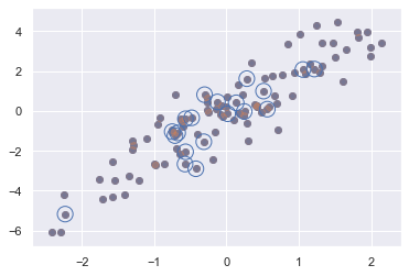
这种方法通常用于快速分割数据,即需要分割训练 / 测试数据集以验证统计模型。
2.7.4 用花哨的索引值修改值
花哨的索引可以被用于获取部分数组,它也可以被用于修改部分数组。
x = np.arange(10)
i = np.array([2, 1, 8, 4])
x[i] = 99
print(x)

x[i] -= 10
print(x)
[ 0 99 99 3 99 5 6 7 99 9]
[ 0 89 89 3 89 5 6 7 89 9]
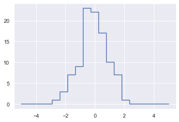
2.7.5 示例:数据区间划分
import numpy as np
import matplotlib.pyplot as plt

np.random.seed(42)
x = np.random.randn(100)
# 手动计算直方图
bins = np.linspace(-5, 5, 20)
counts = np.zeros_like(bins)
# 为每个x找到合适的区间
i = np.searchsorted(bins, x)
# 为每个区间加上1
np.add.at(counts, i, 1)

plt.plot(bins, counts, linestyle='steps')
2.8 数组的排序
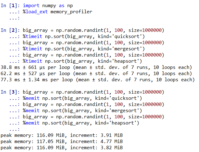
2.8.1 快速排序:np.sort和np.argsort
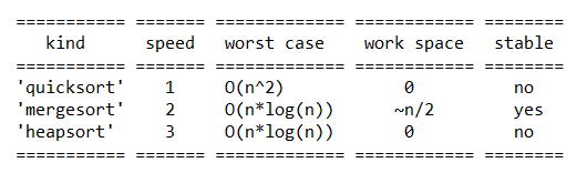
尽管 Python 有内置的 sort 和 sorted 函数可以对列表进行排序,但是 NumPy 的 np.sort 函数实际上效率更高。默认情况下,np.sort 的排序算法是快速排序,其算法复杂度为O [N log N ],另外也可以选择归并排序和堆排序。对于大多数应用场景,默认的快速排序已经足够高效了。
- np.sort:返回排序后的数组;
- np.argsort:返回排序的索引值。
通过 axis 参数,可以沿着多维数组的行或列进行排序。需要记住的是,这种处理方式是将行或列当作独立的数组,任何行或列的值之间的关系将会丢失!
x = np.array([2, 1, 4, 3, 5])

print(np.sort(x))
i = np.argsort(x)
print(i)

rand = np.random.RandomState(42)
X = rand.randint(0, 10, (4, 6))
print(X)

print(np.sort(X, axis=0))
print(np.sort(X, axis=1))
[1 2 3 4 5]
[1 0 3 2 4]
[[6 3 7 4 6 9]
[2 6 7 4 3 7]
[7 2 5 4 1 7]
[5 1 4 0 9 5]]
[[2 1 4 0 1 5]
[5 2 5 4 3 7]
[6 3 7 4 6 7]
[7 6 7 4 9 9]]
[[3 4 6 6 7 9]
[2 3 4 6 7 7]
[1 2 4 5 7 7]
[0 1 4 5 5 9]]
Notes
-----
The various sorting algorithms are characterized by their average speed, worst case performance, work space size, and whether they are stable. A stable sort keeps items with the same key in the same relative
order. The three available algorithms have the following properties:
测试:
2.8.2 部分排序:分隔
有时候我们不希望对整个数组进行排序,仅仅希望找到数组中第 K 小的值,NumPy 的 np.partition 函数提供了该功能。np.partition 函数的输入是数组和数字 K,输出结果是一个新数组,最左边是第 K 小的值,往右是任意顺序的其他值。
x = np.array([7, 2, 3, 1, 6, 5, 4])
print(np.partition(x, 3))
[2 1 3 4 6 5 7]
结果数组中前三个值是数组中最小的三个值,剩下的位置是原始数组剩下的值。在这两个分隔区间中,元素都是任意排列的。
正如 np.argsort 函数计算的是排序的索引值,也有一个 np.argpartition 函数计算的是分隔的索引值。
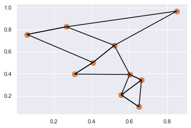
2.8.3 示例:K个最近邻
在二维平面上创建一个有 10 个随机点的集合,并来画出它的散点图。找出距离每个点最近的两个点,并连接。
import numpy as np
import matplotlib.pyplot as plt
import seaborn; seaborn.set() # 设置画图风格

X = np.random.rand(10, 2)
plt.scatter(X[:, 0], X[:, 1], s=100)

dist_sq = np.sum((X[:,np.newaxis,:] - X[np.newaxis,:,:]) ** 2, \
                 axis=-1)

K = 2
nearest_partition = np.argpartition(dist_sq, K + 1, axis=1)
print(nearest_partition)

plt.scatter(X[:, 0], X[:, 1], s=100)
# 将每个点与它的两个最近邻连接
K = 2
for i in range(X.shape[0]):
    for j in nearest_partition[i, :K+1]:
        # 画一条从X[i]到X[j]的线段
        plt.plot(*zip(X[j], X[i]), color='black')
[[0 9 8 3 7 4 2 6 1 5]
[1 6 4 3 2 7 9 5 8 0]
[2 7 3 6 9 4 5 1 8 0]
[3 4 6 7 9 5 1 2 8 0]
[3 6 4 1 7 9 5 2 8 0]
[8 5 7 2 9 3 4 6 1 0]
[6 1 4 3 2 7 9 5 8 0]
[2 7 9 3 4 5 6 1 8 0]
[8 5 9 7 3 2 0 6 1 4]
[3 7 9 8 2 4 6 5 1 0]]
2.9 结构化数据:NumPy的结构化数组
import numpy as np

name = ['Alice', 'Bob', 'Cathy', 'Doug']
age = [25, 45, 37, 19]
weight = [55.0, 85.5, 68.0, 61.5]

data = np.zeros(4, dtype={'names':('name', 'age', 'weight'), \
                          'formats':('U10', 'i4', 'f8')})
print(data.dtype)

data['name'] = name
data['age'] = age
data['weight'] = weight
print(data)

# 获取年龄小于30岁的人的名字
print(data[data['age'] < 30]['name'])
[('name', '<U10'), ('age', '<i4'), ('weight', '<f8')]
[('Alice', 25, 55. ) ('Bob', 45, 85.5) ('Cathy', 37, 68. )
('Doug', 19, 61.5)]
['Alice' 'Doug']
U10 表示“长度不超过 10 的 Unicode 字符串”,i4 表示“4 字节(即 32 比特)整型”,f8 表示“8 字节(即 64 比特)浮点型”。
2.9.1 生成结构化数组
结构化数组的数据类型有多种指定方式,可以用字典或元组列表的方法。
np.dtype({'names':('name', 'age', 'weight'), \
          'formats':('U10', 'i4', 'f8')})
dtype([('name', '<U10'), ('age', '<i4'), ('weight', '<f8')])
np.dtype([('name', 'S10'), ('age', 'i4'), ('weight', 'f8')])
dtype([('name', 'S10'), ('age', '<i4'), ('weight', '<f8')])
第一个(可选)字符是 < 或者 >,分别表示“低字节序”(little endian)和“高字节序”(bid
endian),表示字节(bytes)类型的数据在内存中存放顺序的习惯用法。后一个字符指定的是数据的类型:字符、字节、整型、浮点型,等等(如下表所示)。最后一个字符表示该对象的字节大小。
| Character | Description | Example |
| 'b' | Byte | np.dtype('b') |
| 'i' | Signed integer | np.dtype('i4') == np.int32 |
| 'u' | Unsigned integer | np.dtype('u1') == np.uint8 |
| 'f' | Floating point | np.dtype('f8') == np.int64 |
| 'c' | Complex floating point | np.dtype('c16') == np.complex128 |
| 'S', 'a' | String | np.dtype('S5') |
| 'U' | Unicode string | np.dtype('U') == np.str_ |
| 'V' | Raw data (void) | np.dtype('V') == np.void |
2.9.2 更高级的符合类型
创建一个数据类型,该数据类型用 mat 组件包含一个 3×3的浮点矩阵。
tp = np.dtype([('id', 'i8'), ('mat', 'f8', (3, 3))])
X = np.zeros(1, dtype=tp)
print(X[0])
print(X['mat'][0])
(0, [[0., 0., 0.], [0., 0., 0.], [0., 0., 0.]])
[[0. 0. 0.]
[0. 0. 0.]
[0. 0. 0.]]
2.9.3 记录数组:结构化数组的扭转
NumPy 还提供了 np.recarray 类。它和前面介绍的结构化数组几乎相同,但是它有一个独特的特征:域可以像属性一样获取,而不是像字典的键那样获取。前面的例子通过以下代码获取年龄。
print(data['age'])

data_rec = data.view(np.recarray)
print(data_rec.age)
[25 45 37 19]
[25 45 37 19]

 浙公网安备 33010602011771号