MATLAB神经网络（2） BP神经网络的非线性系统建模——非线性函数拟合

2.1 案例背景

在工程应用中经常会遇到一些复杂的非线性系统，这些系统状态方程复杂，难以用数学方法准确建模。在这种情况下，可以建立BP神经网络表达这些非线性系统。该方法把未知系统看成是一个黑箱，首先用系统输入输出数据训练BP神经网络，使网络能够表达该未知函数，然后用训练好的BP神经网络预测系统输出。

本章拟合的非线性函数为\[y = {x_1}^2 + {x_2}^2\]该函数的图形如下图所示。

t=-5:0.1:5;
[x1,x2] =meshgrid(t);
y=x1.^2+x2.^2;
surfc(x1,x2,y);
shading interp
xlabel('x1');
ylabel('x2');
zlabel('y');
title('非线性函数');

2.2 模型建立

神经网络结构：2-5-1

从非线性函数中随机得到2000组输入输出数据，从中随机选择1900 组作为训练数据，用于网络训练，100组作为测试数据，用于测试网络的拟合性能。

2.3 MATLAB实现

2.3.1 BP神经网络工具箱函数

newff

BP神经网络参数设置函数。

net=newff(P, T, S, TF, BTF, BLF, PF, IPF, OPF, DDF)

• P：输入数据矩阵；
• T：输出数据矩阵；
• S：隐含层节点数；
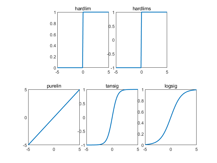
• TF：结点传递函数。包括硬限幅传递函数hardlim、对称硬限幅传递函数hardlims、线性传递函数purelin、正切 型传递函数tansig、对数型传递函数logsig；

x=-5:0.1:5;
subplot(2,6,[2,3]);
y=hardlim(x);
plot(x,y,'LineWidth',1.5);
title('hardlim');
subplot(2,6,[4,5]);
y=hardlims(x);
plot(x,y,'LineWidth',1.5);
title('hardlims');
subplot(2,6,[7,8]);
y=purelin(x);
plot(x,y,'LineWidth',1.5);
title('purelin');
subplot(2,6,[9,10]);
y=tansig(x);
plot(x,y,'LineWidth',1.5);
title('tansig');
subplot(2,6,[11,12]);
y=logsig(x);
plot(x,y,'LineWidth',1.5);
title('logsig');

• BTF：训练函数。包括梯度下降BP算法训练函数traingd、动量反传的梯度下降BP算法训练函数traingdm、动态自适应学习率的梯度下降BP算法训练函数traingda、动量反传和动态自适应学习率的梯度下降BP算法训练函数traingdx、Levenberg_Marquardt的BP算法训练函数trainlm；
• BLF：网络学习函数。包括BP学习规则learngd、带动量项的BP学习规则learngdm；
• PF：性能分析函数，包括均值绝对误差性能分析函数mae、均方差性能分析函数mse；
• IPF：输入处理函数；
• OPF：输出处理函数；
• DDF：验证数据划分函数。

一般在使用过程中设置前面6个参数，后面4个参数采用系统默认参数。

train

用训练数据训练BP神经网络。

[net, tr]=train(NET, X, T, Pi, Ai)

• NET：待训练网络；
• X：输入数据矩阵；
• T输出数据矩阵；
• Pi：初始化输入层条件；
• Ai：初始化输出层条件；
• net：训练好的网络；
• 训练过程记录。

sim

BP神经网络预测函数。

y=sim(net, x)

• net：训练好的网络；
• x：输入数据；
• y：网络预测数据。

2.3.2 数据选择和归一化

%% 基于BP神经网络的预测算法

%% 清空环境变量
clc
clear

%% 训练数据预测数据提取及归一化
input=10*randn(2,2000);
output=sum(input.*input);

%从1到2000间随机排序
k=rand(1,2000);
[m,n]=sort(k);

%找出训练数据和预测数据
input_train=input(:,n(1:1900));
output_train=output(n(1:1900));
input_test=input(:,n(1901:2000));
output_test=output(n(1901:2000));

%选连样本输入输出数据归一化
[inputn,inputps]=mapminmax(input_train);
[outputn,outputps]=mapminmax(output_train);

2.3.3 BP神经网络训练

%% BP网络训练
% %初始化网络结构
net=newff(inputn,outputn,5);

% 配置网络参数（迭代次数，学习率，目标）
net.trainParam.epochs=100;
net.trainParam.lr=0.1;
net.trainParam.goal=0.00004;

%网络训练
net=train(net,inputn,outputn);

2.3.4 BP神经网络预测

%% BP网络预测
%预测数据归一化
inputn_test=mapminmax('apply',input_test,inputps);
 
%网络预测输出
an=sim(net,inputn_test);
 
%网络输出反归一化
BPoutput=mapminmax('reverse',an,outputps);

2.3.5 结果分析

%% 结果分析
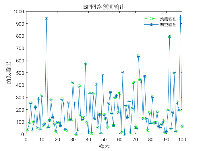
figure(1)
plot(BPoutput,':og')
hold on
plot(output_test,'-*');
legend('预测输出','期望输出')
title('BP网络预测输出','fontsize',12)
ylabel('函数输出','fontsize',12)
xlabel('样本','fontsize',12)

%预测误差
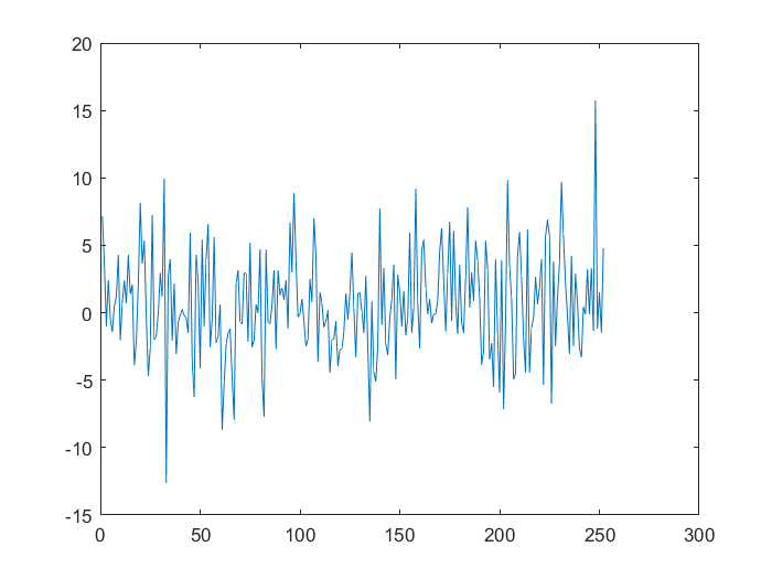
error=BPoutput-output_test;

figure(2)
plot(error,'-*')
title('BP网络预测误差','fontsize',12)
ylabel('误差','fontsize',12)
xlabel('样本','fontsize',12)

figure(3)
plot((BPoutput-output_test)./output_test,'-*');
title('神经网络预测误差百分比')

% 计算平均绝对百分比误差(mean absolute percentage error)
MAPE=mean(abs(BPoutput-output_test)./output_test)

2.4 扩展

2.4.1 多隐含层BP神经网络

net=newff(P, T, S, TF, BTF, BLF, PF, IPF, OPF, DDF)

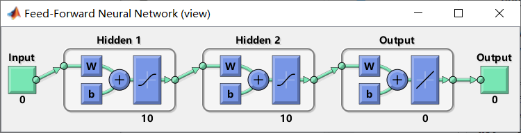
S可为向量，如[5,5]表示该BP神经网络为双层，每个隐含层的节点数都是5。

 

 

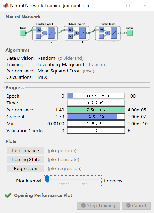
• Neural Network：神经网络结构，输入、中间层、输出维度。

• Data Division：数据划分算法；
• Training：训练算法；
• Performance：误差算法；
• Calculations：编译算法。

• Epoch：迭代次数；
• Time：训练时间；
• Performance：误差；
• Gradient：梯度；
• Mu：阻尼因子；
• Validation Checks：泛化能力检查。

• Performance：误差图示；
• Training State：训练状况图示；
• Regression：回归曲线图示；
• Plot Interval：绘图刻度。

2.4.2 隐含层节点数

对复杂问题来说，网络预测误差随节点数增加一般呈现先减少后增加的趋势。

2.4.3 训练数据对预测精度的影响

缺乏训练数据可能使BP神经网络得不到充分训练，预测值和期望值之间误差较大。

2.4.4 节点转移函数

一般隐含层选择logsig或tansig，输出层选择tansig或purelin。

2.4.5 网络拟合的局限性

BP神经网络虽然具有较好的拟合能力，但其拟合能力不是绝对的，对于一些复杂系统，BP 神经网络预测结果会存在较大误差。

2.5 MATLAB doc

Feedforward networks consist of a series of layers. The first layer has a connection from the network input. Each subsequent layer has a connection from the previous layer. The final layer produces the network’s output.

Feedforward networks can be used for any kind of input to output mapping. A feedforward network with one hidden layer and enough neurons in the hidden layers, can fit any finite input-output mapping problem.

• feedforwardnet(hiddenSizes,trainFcn)

This following example loads a dataset that maps anatomical measurements x to body fat percentages t. A feedforward network with 10 neurons is created and trained on that data, then simulated.

[x,t] =  bodyfat_dataset;  
net = feedforwardnet([10,10]);
view(net);
net = train(net,x,t);
y = net(x);
plot((y-t))