Matlab绘图

基础绘图

图线的绘制与装饰

使用plot()和fplot函数绘制图线

在MATLAB中,使用plot()函数绘制图线,其语法为:

plot(x,y,LineSpec)

各参数意义如下:

• x: 图线上点的x坐标
• y: 图线上点的y坐标
• LineSpec: 图线的线条设定,三个指定线型,标记符号和颜色的设定符组成一个字符串,设定符不区分先后.具体细节请参考官方文档.

线型设定符	线型	标记设定符	标记	颜色设定符	颜色
-	实线（默认）	o	圆圈	y	黄色
--	虚线	+	加号	m	品红色
:	点线	*	星号	c	青蓝色
-.	点划线	.	点	r	红色
		x	叉号	g	绿色
		s	方形	b	蓝色
		d	菱形	w	白色
		^	上三角	k	黑色
		v	下三角
		>	右三角
		<	左三角
		p	五角形
		h	六角形

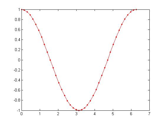
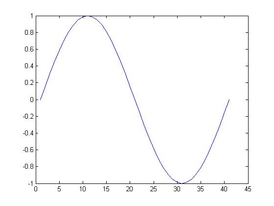
下面例子演示了绘制 \((0,2\pi)\) 内余弦函数的图像:

x = 0:pi/20:2*pi;
y = cos(x);
plot(x, y, 'r.-')

fplot的用法见官方文档.

装饰图线

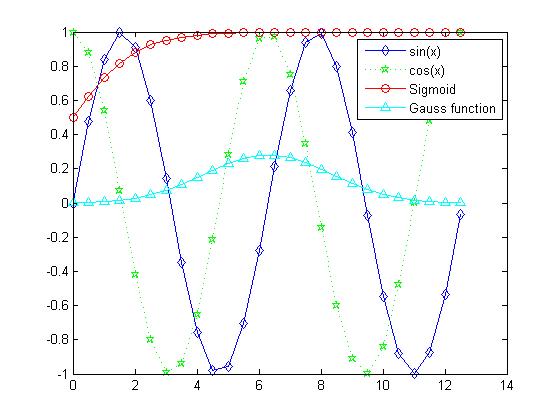
使用legend()函数为图片增加图例, legend(label1, ..., labelN)函数可以为图片添加图例.

x=0:0.5:4*pi;
y=sin(x); h=cos(x); w=1./(1+exp(-x)); g=(1/(2*pi*2)^0.5).*exp((-1.*(x-2*pi).^2)./(2*2^2));
plot(x,y,'bd-' ,x,h,'gp:',x,w,'ro-' ,x,g,'c^-');		% 绘制多条图线
legend('sin(x)','cos(x)','Sigmoid','Gauss function');	% 添加图例

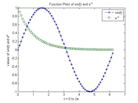
使用title()和*label()为图片增加标题和标签

x = 0:0.1:2*pi; y1 = sin(x); y2 = exp(-x);
plot(x, y1, '--*', x, y2, ':o');
xlabel('t = 0 to 2\pi');
ylabel('values of sin(t) and e^{-x}')
title('Function Plots of sin(t) and e^{-x}');
legend('sin(t)','e^{-x}');

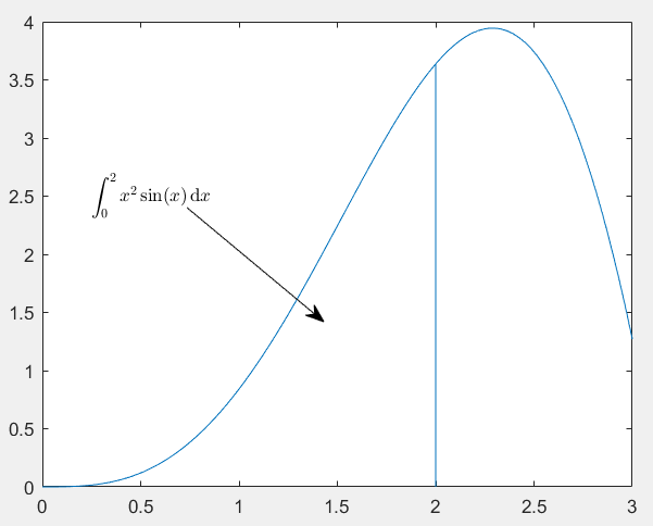
使用text()和annotation()为图片增加注解

x = linspace(0,3); y = x.^2.*sin(x); plot(x,y);
line([2,2],[0,2^2*sin(2)]);
str = '$$ \int_{0}^{2} x^2\sin(x) \,{\rm d}x $$';
text(0.25,2.5,str,'Interpreter','latex');
annotation('arrow','X',[0.32,0.5],'Y',[0.6,0.4]); 

控制坐标轴,边框与网格

使用下列命令可以控制坐标轴,边框与网格.

命令	作用
grid on/off	设置网格可见性
box on/off	设置边框可见性
axis on/off	设置坐标轴可见性
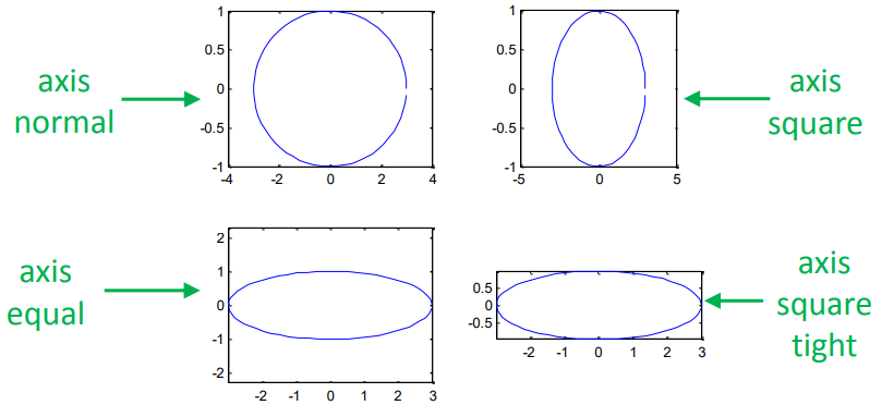
axis normal	还原默认行为,将图框纵横比模式和数据纵横比模式的属性设置为自动
axis square	使用相同长度的坐标轴线,相应调整数据单位之间的增量
axis equal	沿每个坐标轴使用相同的数据单位长度
axis tight	将坐标轴范围设置为等同于数据范围,使轴框紧密围绕数据

下面的例子演示axis命令的效果:

t = 0:0.1:2*pi; x = 3*cos(t); y = sin(t);
subplot(2, 2, 1); plot(x, y); axis normal
subplot(2, 2, 2); plot(x, y); axis square
subplot(2, 2, 3); plot(x, y); axis equal
subplot(2, 2, 4); plot(x, y); axis equal tight

绘制多条图线

在一个图像上绘制多条图线

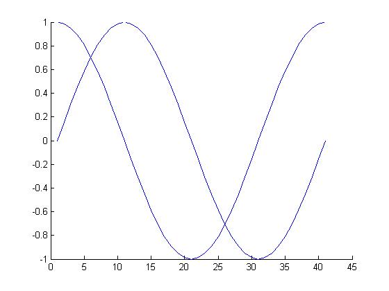
默认情况下,每次执行plot()函数都会清除上一次绘图的结果,多次执行plot()只会保留最后一次绘制的图形.

plot(cos(0:pi/20:2*pi));
plot(sin(0:pi/20:2*pi));

我们可以使用hold on和hold off命令控制绘图区域的刷新,使得多个绘图结果同时保留在绘图区域中.

hold on		% 提起画笔,开始绘制一组图片			
plot(cos(0:pi/20:2*pi));
plot(sin(0:pi/20:2*pi));
hold off	% 放下画笔,该组图片绘制完毕

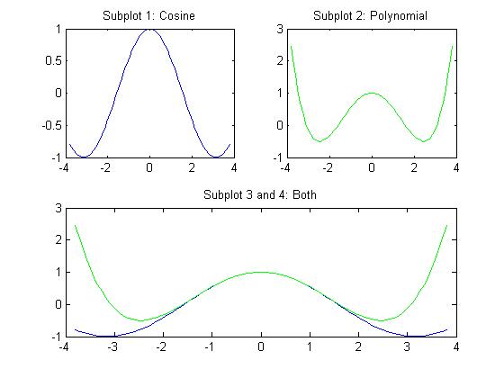
在一个窗口内绘制多个图像

使用subplot()函数可以在一个窗口内绘制多个图像.其语法为:

subplot(m,n,p)

该命令表示将当前图窗划分为m×n个网格,并在第p个网格内绘制图像.

示例如下:

subplot(2,2,1);
x = linspace(-3.8,3.8);
y_cos = cos(x);
plot(x,y_cos);
title('Subplot 1: Cosine')

subplot(2,2,2);
y_poly = 1 - x.^2./2 + x.^4./24;
plot(x,y_poly,'g');
title('Subplot 2: Polynomial')

subplot(2,2,[3,4]);
plot(x,y_cos,'b',x,y_poly,'g');
title('Subplot 3 and 4: Both')

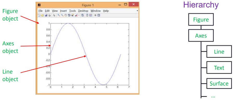
图形对象的操作

在MATLAB中,图形都是以对象的形式储存在内存中,通过获取其图形句柄可以对其进行操作.

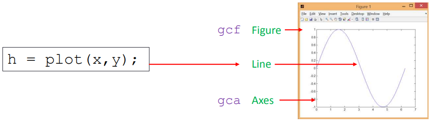
获取图形句柄

图形句柄本质上就是一个浮点数,可以唯一确定一个图形对象.下面几个函数用于获取图形句柄.

Function	Purpose
gca()	获取当前坐标轴的句柄
gcf()	获取当前图像的句柄
allchild(handle_list)	获取该对象的所有子对象的句柄
ancestor(h,type)	获取对象最近的type类型的祖先节点
delete(h)	删除某对象
findall(handle_list)	获取该对象的后代对象

所有绘图函数也会返回图形对象的句柄.

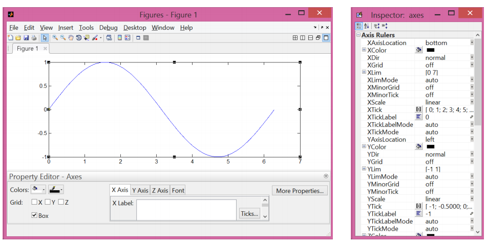
通过图形句柄操作图形属性

使用get()和set()函数可以对图形对象的属性进行访问和修改.访问官方文档可以查看所有图形对象的属性.

• set(H,Name,Value)
• v = get(h,propertyName)

下面两个例子演示使用图形句柄操作图形对象:

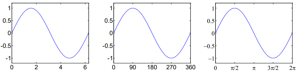
1. 改变坐标轴属性

% 第一张图
set(gca, 'FontSize', 25);

% 第二张图
set(gca, 'XTick', 0:pi/2:2*pi);
set(gca, 'XTickLabel', 0:90:360);

% 第三张图
set(gca, 'FontName', 'symbol');
set(gca, 'XTickLabel', {'0', 'p/2', 'p', '3p/2', '2p'});

2. 改变线型

h = plot(x,y); 
set(h, 'LineStyle','-.', ...
	'LineWidth', 7.0, ...
	'Color', 'g');

将图形保存到文件

使用saveas(fig,filename)命令可以将图形对象保存到文件中,其中fig为图形句柄,filname为文件名.

saveas(gcf, 'myfigure.png')

使用saveas()函数将图像保存成位图时,会发生失真.要精确控制生成图片的质量,可以使用print()函数,见官方文档.

绘制高级图表

二维图表

折线图

函数	图形描述
loglog()	x轴和y轴都取对数坐标
semilogx()	x轴取对数坐标,y轴取线性坐标
semilogy()	x轴取线性坐标,y轴取对数坐标
plotyy()	带有两套y坐标轴的线性坐标系
ploar()	极坐标系

对数坐标系图线

下面例子演示对数坐标系图线:

x = logspace(-1,1,100); y = x.^2;

subplot(2,2,1);
plot(x,y);
title('Plot');

subplot(2,2,2);
semilogx(x,y);
title('Semilogx');

subplot(2,2,3);
semilogy(x,y);
title('Semilogy');

subplot(2,2,4);
loglog(x, y);
title('Loglog'); 

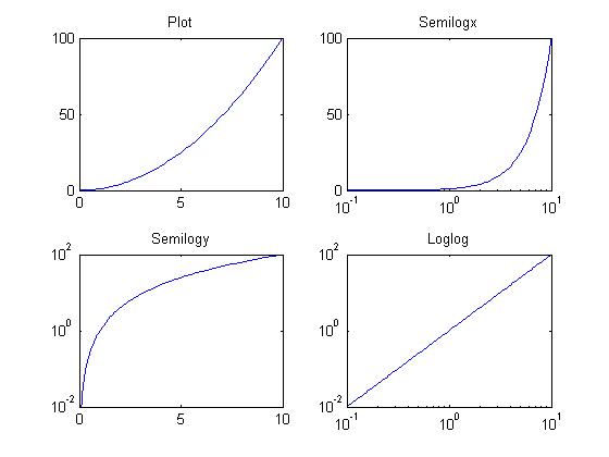
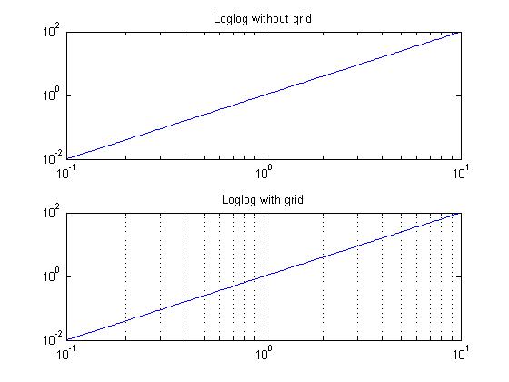
对数坐标系可以加上网格,以区分线性坐标系与对数坐标系.

set(gca, 'XGrid','on');

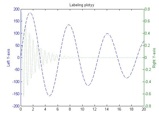
双y轴图线

plotyy()的返回值为数组[ax,hlines1,hlines2],其中:

• ax为一个向量,保存两个坐标系对象的句柄.
• hlines1和hlines2分别为两个图线的句柄.

x = 0:0.01:20;
y1 = 200*exp(-0.05*x).*sin(x);
y2 = 0.8*exp(-0.5*x).*sin(10*x);
[AX,H1,H2] = plotyy(x,y1,x,y2);
set(get(AX(1),'Ylabel'),'String','Left Y-axis')
set(get(AX(2),'Ylabel'),'String','Right Y-axis')
title('Labeling plotyy');
set(H1,'LineStyle','--'); set(H2,'LineStyle',':');

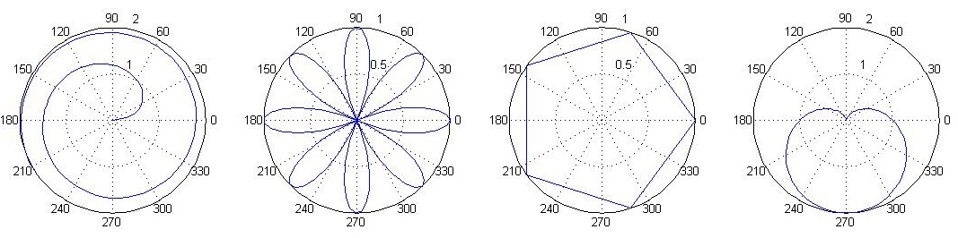
极坐标图线

% 螺旋线
x = 1:100; theta = x/10; r = log10(x);
subplot(1,4,1); polar(theta,r);

% 花瓣
theta = linspace(0, 2*pi); r = cos(4*theta);
subplot(1,4,2); polar(theta, r);

% 五边形
theta = linspace(0, 2*pi, 6); r = ones(1,length(theta));
subplot(1,4,3); polar(theta,r);

% 心形线
theta = linspace(0, 2*pi); r = 1-sin(theta);
subplot(1,4,4); polar(theta , r);

统计图表

函数	图形描述
hist()	直方图
bar()	二维柱状图
pie()	饼图
stairs()	阶梯图
stem()	针状图

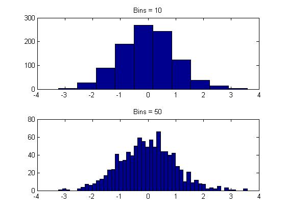
直方图

使用hist()绘制直方图,语法如下:

hist(x,nbins)

其中:

• x表示原始数据
• nbins表示分组的个数

x = randn(1,1000);
subplot(2,1,1);
hist(x,10);
title('Bins = 10');
subplot(2,1,2);
hist(x,50);
title('Bins = 50');

柱状图

使用bar()和bar3()函数分别绘制二维和三维直方图

x = [1 2 5 4 8]; y = [x;1:5];
subplot(1,3,1); bar(x); title('A bargraph of vector x');
subplot(1,3,2); bar(y); title('A bargraph of vector y');
subplot(1,3,3); bar3(y); title('A 3D bargraph');

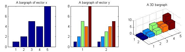
hist主要用于查看变量的频率分布,而bar主要用于查看分立的量的统计结果.

使用barh()函数可以绘制纵向排列的柱状图

x = [1 2 5 4 8];
y = [x;1:5];
barh(y);
title('Horizontal');

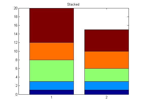
向bar()传入'stack'参数可以让柱状图以堆栈的形式画出.

x = [1 2 5 4 8];
y = [x;1:5];
bar(y,'stacked');
title('Stacked');

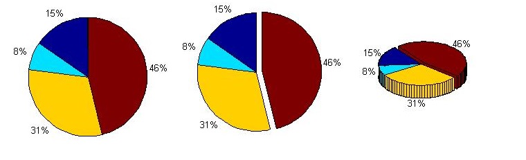
饼图

使用pie()和pie3()可以绘制二维和三维的饼图.向其传入一个bool向量表示每一部分扇区是否偏移.

a = [10 5 20 30];
subplot(1,3,1); pie(a);
subplot(1,3,2); pie(a, [0,0,0,1]);
subplot(1,3,3); pie3(a, [0,0,0,1]);

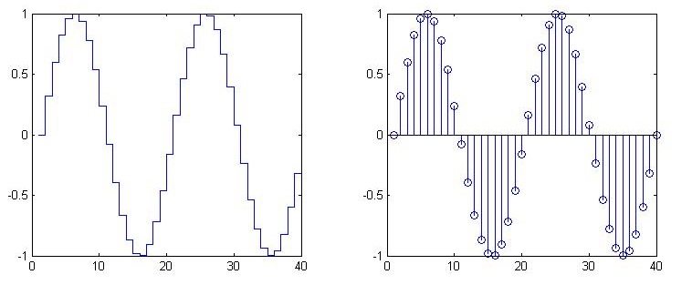
阶梯图和针状图:绘制离散数字序列

stairs()和stem()函数分别用来绘制阶梯图和针状图,用于表示离散数字序列.

x = linspace(0, 4*pi, 40); y = sin(x);
subplot(1,2,1); stairs(y);
subplot(1,2,2); stem(y);

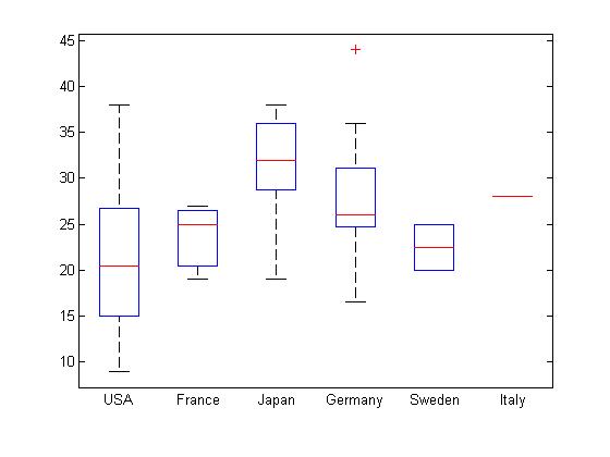
其它统计图表

boxplot()

load carsmall
boxplot(MPG, Origin);

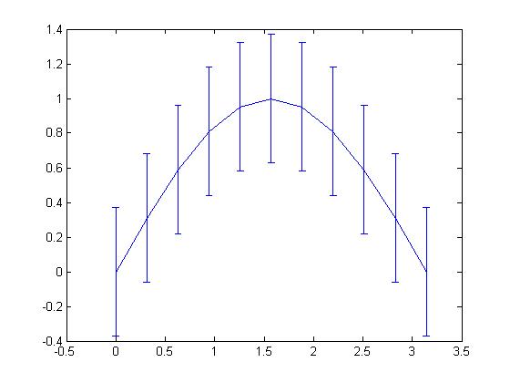
errorbar()

errorbar()
x=0:pi/10:pi; y=sin(x);
e=std(y)*ones(size(x));
errorbar(x,y,e)

绘制图形

MATLAB也可以绘制简单的图形,使用fill()函数可以对区域进行填充.

t =(1:2:15)'*pi/8; x = sin(t); y = cos(t);
fill(x,y,'r'); axis square off;
text(0,0,'STOP','Color', ...
	'w', 'FontSize', 80, ... 
	'FontWeight','bold', ...
	'HorizontalAlignment', 'center');

三维图表

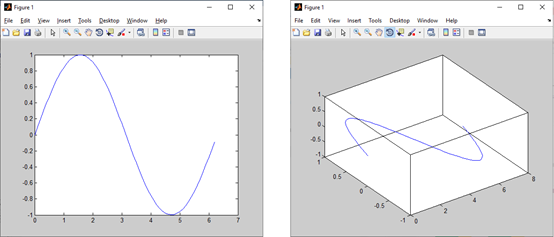
二维图与三维图间的关系

二维图转为三维图

在MATLAB中,所有的图都是三维图,二维图只不过是三维图的一个投影.点击图形窗口的Rotate 3D按钮,即可通过鼠标拖拽查看该图形的三维视图.

三维图转换为二维图

使用imagesc()函数可以将三维图转换为二维俯视图,通过点的颜色指示高度.

[x, y] = meshgrid(-3:.2:3,-3:.2:3); z = x.^2 + x.*y + y.^2; 

subplot(1, 2, 1)
surf(x, y, z); 

subplot(1, 2, 2)
imagesc(z);

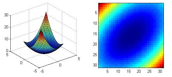
使用colorbar命令可以在生成的二维图上增加颜色与高度间对应关系的图例,使用colormap命令可以改变配色方案.具体细节请参考官方文档.

三维图的绘制

使用meshgrid()生成二维网格

我们对一个二维网格矩阵应用函数 \(z = f ( x , y )\) 才能得到三维图形,因此在得到三维数据之前我们应当使用meshgrid()函数生成二维网格矩阵.

meshgrid()函数将输入的两个向量进行相应的行扩充和列扩充以得到两个增广矩阵,对该矩阵可应用二元函数.

x = -2:1:2;
y = -2:1:2;
[X,Y] = meshgrid(x,y)
Z = X.^2 + Y.^2

我们得到了生成的二维网格矩阵如下:

X =
    -2    -1     0     1     2
    -2    -1     0     1     2
    -2    -1     0     1     2
    -2    -1     0     1     2
    -2    -1     0     1     2


Y =
    -2    -2    -2    -2    -2
    -1    -1    -1    -1    -1
     0     0     0     0     0
     1     1     1     1     1
     2     2     2     2     2
     
Z =
     8     5     4     5     8
     5     2     1     2     5
     4     1     0     1     4
     5     2     1     2     5
     8     5     4     5     8

绘制三维线

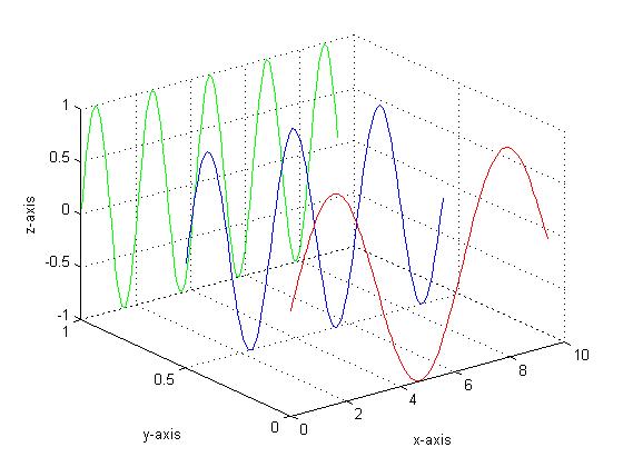
使用plot3()函数即可绘制三维面,输入应为三个向量.

x=0:0.1:3*pi; z1=sin(x); z2=sin(2.*x); z3=sin(3.*x);
y1=zeros(size(x)); y3=ones(size(x)); y2=y3./2;
plot3(x,y1,z1,'r',x,y2,z2,'b',x,y3,z3,'g'); grid on;
xlabel('x-axis'); ylabel('y-axis'); zlabel('z-axis');

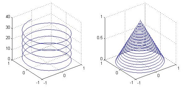
下面例子绘制了两个螺旋线:

subplot(1, 2, 1)
t = 0:pi/50:10*pi;
plot3(sin(t),cos(t),t)
grid on; axis square;

subplot(1, 2, 2)
turns = 40*pi;
t = linspace(0,turns,4000);
x = cos(t).*(turns-t)./turns;
y = sin(t).*(turns-t)./turns;
z = t./turns;
plot3(x,y,z); grid on;

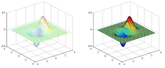
绘制三维面

使用mesh()和surf()命令可以绘制三维面,前者不会填充网格而后者会.

x = -3.5:0.2:3.5; y = -3.5:0.2:3.5;
[X,Y] = meshgrid(x,y);
Z = X.*exp(-X.^2-Y.^2);
subplot(1,2,1); mesh(X,Y,Z);
subplot(1,2,2); surf(X,Y,Z);

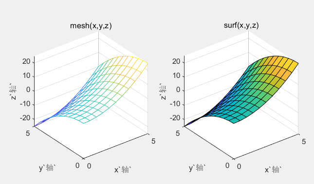
绘制 \(z = x^2 − y^2\) 的图像，其中 \(x\) 和 \(y\) 都位于 \([0, 5]\) 之间.

[x,y] = meshgrid(linspace(0,5,11));
z = x.^2 - y.^2;
subplot(1,2,1); 
mesh(x,y,z);
xlabel('x`轴`');  ylabel('y`轴`');  zlabel('z`轴`');
axis vis3d; 
title('mesh(x,y,z)');

subplot(1,2,2);
surf(x,y,z);  
xlabel('x`轴`');  ylabel('y`轴`');  zlabel('z`轴`'); 
axis vis3d;
title('surf(x,y,z)')

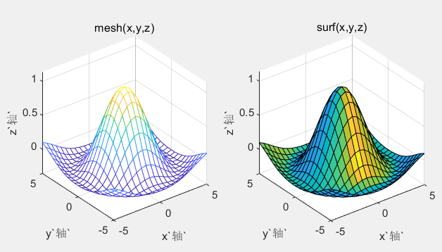
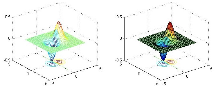
绘制 \(\displaystyle z=\frac{\sin\left(\sqrt{x^2+y^2}\right)}{\sqrt{x^2+y^2}}\) 的图形，其中 \(x\) 和 \(y\) 都位于 \([-5,5]\) 之间.

[x,y] = meshgrid(-5:0.5:5); % 快速生成网格所需的数据	
tem = sqrt(x.^2+y.^2)+1e-12;   % tem=sqrt(x.^2+y.^2)
% 在后面加上一个非常非常小的数字: 1e-12 = 10^(-12) ,当然你也可以单独找到值为0的地方对其修改
z = sin(tem)./tem; % 如果不对tem处理，那么z的最中间的一个值 0/0 = NaN
subplot(1,2,1)
mesh(x,y,z)
xlabel('x`轴`');  ylabel('y`轴`');  zlabel('z`轴`'); 
axis vis3d 
title('mesh(x,y,z)')

subplot(1,2,2)
surfl(x,y,z)  % (X(j), Y(i), Z(i,j))`是线框网格线的交点` % surfl `函数:加上了灯光效果,看起来自然点`
xlabel('x`轴`');  ylabel('y`轴`');  zlabel('z`轴`');  
axis vis3d 
title('surf(x,y,z)')

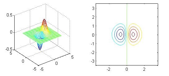
绘制三维图形的等高线

使用contour()和contourf()函数可以绘制三维图形的等高线,前者不会填充网格而后者会.

x = -3.5:0.2:3.5;
y = -3.5:0.2:3.5;
[X,Y] = meshgrid(x,y);
Z = X.*exp(-X.^2-Y.^2);

subplot(1,2,1);
mesh(X,Y,Z); axis square;
subplot(1,2,2);
contour(X,Y,Z); axis square;

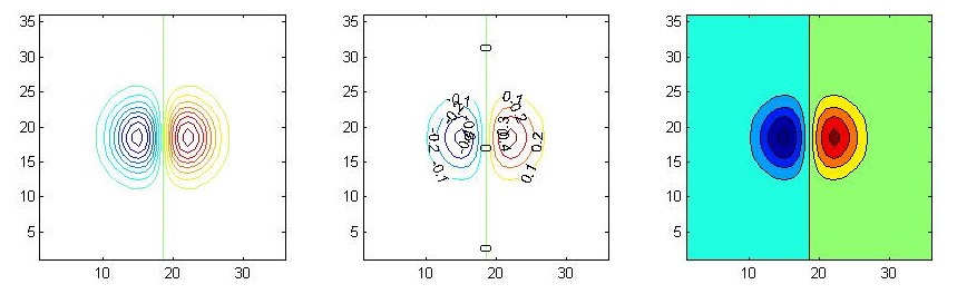
向contour()函数传入参数或操作图形句柄可以改变图像的细节:

x = -3.5:0.2:3.5; y = -3.5:0.2:3.5;
[X,Y] = meshgrid(x,y); Z = X.*exp(-X.^2-Y.^2);

subplot(1,3,1); contour(Z,[-.45:.05:.45]); axis square;
subplot(1,3,2); [C,h] = contour(Z); clabel(C,h); axis square;
subplot(1,3,3); contourf(Z); axis square;

使用meshc()和surfc()函数可以在绘制三维图形时绘制其等高线.

x = -3.5:0.2:3.5; y = -3.5:0.2:3.5;
[X,Y] = meshgrid(x,y); Z = X.*exp(-X.^2-Y.^2);

subplot(1,2,1); meshc(X,Y,Z);
subplot(1,2,2); surfc(X,Y,Z);

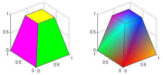
绘制三维体

使用patch()函数可以绘制三维体.

v = [0 0 0; 1 0 0 ; 1 1 0; 0 1 0; 0.25 0.25 1; 0.75 0.25 1; 0.75 0.75 1; 0.25 0.75 1];
f = [1 2 3 4; 5 6 7 8; 1 2 6 5; 2 3 7 6; 3 4 8 7; 4 1 5 8];

subplot(1,2,1); 
patch('Vertices', v, 'Faces', f, 'FaceVertexCData', hsv(6), 'FaceColor', 'flat');
view(3); axis square tight; grid on;

subplot(1,2,2); 
patch('Vertices', v, 'Faces', f, 'FaceVertexCData', hsv(8), 'FaceColor','interp');
view(3); axis square tight; grid on

三维图的视角与打光

调整视角

使用view()函数可以调整视角,view()函数接受两个浮点型参数,分别表示两个方位角azimuth和elevation.

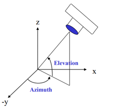
sphere(50); shading flat;
material shiny;
axis vis3d off;
view(-45,20);

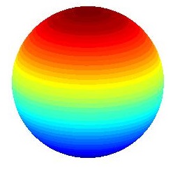
调整打光

使用light()函数可以对三维图形进行打光,并返回光源的句柄.

[X, Y, Z] = sphere(64); h = surf(X, Y, Z);
axis square vis3d off;
reds = zeros(256, 3); reds(:, 1) = (0:256.-1)/255;
colormap(reds); shading interp; lighting phong;
set(h, 'AmbientStrength', 0.75, 'DiffuseStrength', 0.5);
L1 = light('Position', [-1, -1, -1])

通过对光源的句柄进行操作可以修改光源的属性

set(L1, 'Position', [-1, -1, 1]);
set(L1, 'Color', 'g');

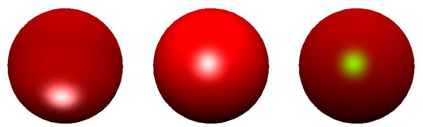
一些示例图

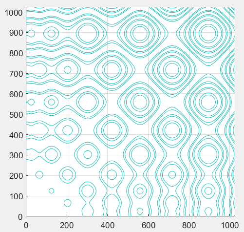
鱼形曲线

hold on
axis equal
grid on
X=0:1:1023;
Y=0:1:1023;
[gridX,gridY]=meshgrid(X,Y);
FishPatternFcn=@(x,y)mod(abs(x.*sin(sqrt(x))+y.*sin(sqrt(y))).*pi./1024,1);
contour(gridX,gridY,FishPatternFcn(gridX,gridY),[0.7,0.7])

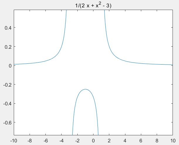
画囧

syms x;
g=1/(x^2+2*x-3);
ezplot(g,-10,10);

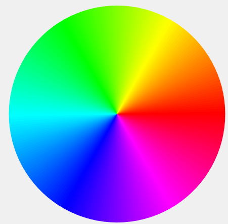
光盘

t = (0:.02:2)*pi;
r = 0:.02:1; %r = 0.3:.02:1; 
pcolor(cos(t)'*r,sin(t)'*r,t'*(r==r))
colormap(hsv(256)), shading interp, axis image off
%ezsurf('r*cos(t)','r*sin(t)','t',[0 1 0 2*pi])
%colormap(hsv(256)),shading interp,view(2), axis imae off

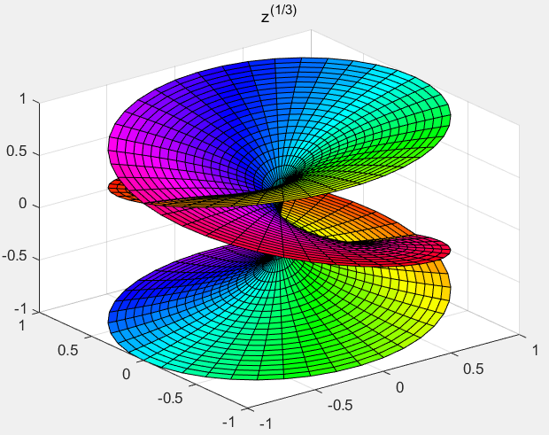
黎曼曲面的平面效果

cplxdemo;

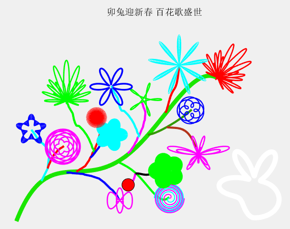
百花争艳图

% By ZFN  2011.3
hf=figure('name','百花争艳图');
axis([0 22 0 16]);
axis equal
title('卯兔迎新春 百花歌盛世');
axis off
hold on
 

%%%%%%%%%%%%%%%%%%%%%%%%%%%%%%%%  画的树干
gx=[0 1 2 3 4 4.2 5 5.1 6 7 8 8.2 8.7 9 9.2 10 10.5 11 11.5 11.7 12.3 12.5 13 13.5 14];
gy=[0 1.8 3.1 3.3 3.8 3.9 4 4.05 4.1 4.3 4.55 4.6 4.75 5 5.65 6.2 6.8 7.4 8 8.4 9 9.3 9.87 10.25 10.8];


p=polyfit(gx,gy,4);
gxx=linspace(0,16,100);
gyy=polyval(p,gxx);

plot(gxx,gyy,'linewidth',5,'color',[0.1 0.9 0]);

c1x=[2 2.3 2.5 2.6 2.55 2.5 2.4 2.3 2.2 2.1 1.8 1.5 1.2];
c1y=[3.1 3.7 4.1 5 5.4 5.6 5.8 5.9 6 6.1 6.3 6.8 7.2];
plot(c1x,c1y,'linewidth',2.5,'color','c');

c1x1=[2.5 2.6 2.7 2.8 2.9 3 3.1 3.2 3.3 3.4 3.5 3.6 3.7 3.8];
c1y1=[4.1 4.4 4.6 4.85 5 5.2 5.3 5.4 5.55 5.6 5.7 5.76 5.82 5.9];
plot(c1x1,c1y1,'linewidth',2.5,'color','r');


c2x=[4 4.3 4.4 4.5 5 5.1 5.3 5.5 5.6 5.8 6 6.3 6.6 6.8 7 7.1 7.2 7.3 7.5 7.7 7.9 8 8.1 8.2 ];
c2y=[3.78 3.78 3.75 3.73 3.7 3.68 3.67 3.6 3.58 3.54 3.5 3.4 3.3 3.15 3 2.9 2.8 2.7 2.5 2.35 2.1 2 1.8 1.6];
plot(c2x,c2y,'linewidth',2.5,'color','b');

c3x=[4.8 5.1 5.2 5.3 5.5 5.7 5.8 5.9 6 6.1 6.2 6.4 6.5 6.6 6.65 6.66 6.67 6.68 6.69 6.7 6.65 6.6 6.55 6.5 6.45 6.4];
c3y=[3.85 4.05 4.1 4.17 4.3 4.6 4.74 4.96 5.1 5.4 5.5 6 6.2 6.66 6.76 6.86 7 7.1 7.2 7.4 7.55 7.68 7.8 8 8.1 8.2];
plot(c3x,c3y,'linewidth',2.5,'color','r');

c3x1=[6.1 6.2 6.17 6.15 6.1 6.05 6 5.9 5.8 5.6 5.5 5.4 5.3 5.2 5.1 5 4.9 4.8 4.7 4.6 4.5 4.2 4];
c3y1=[5.4 5.5 5.6 5.65 5.7 5.8 6 6.2 6.45 6.8 6.93 7.08 7.2 7.3 7.4 7.5 7.51 7.52 7.7 8 8.5 9 9.5];
plot(c3x1,c3y1,'linewidth',2.5,'color','g');

c3x2=[5.9 6 6.1 6.2 6.4 6.5 6.6 6.7 6.8 6.9 7 7.1 7.2 7.3 7.4 7.5 7.6];
c3y2=[4.96 5.05 5.15 5.27 5.54 5.67 5.8 6 6.08 6.2 6.3 6.4 6.5 6.62 6.7 6.8 6.85];
plot(c3x2,c3y2,'linewidth',2.5,'color','b');

%c5x=c3x+3.6;
%c5y=c3y+1.2;
%plot(c5x,c5y); 

c5x=[5.3 5.5 5.7 5.8 5.9 6 6.1 6.2 6.4 6.5 6.6 6.65 6.66 6.67 6.68 6.69 6.7 6.65 6.6 6.55 6.5 6.45 6.4]+3.6;
c5y=[4.11 4.3 4.6 4.74 4.96 5.1 5.4 5.5 6 6.2 6.66 6.76 6.86 7 7.1 7.2 7.4 7.55 7.68 7.8 8 8.1 8.2]+1.2;
plot(c5x,c5y,'linewidth',2.5,'color','m');

c5x1=c3x1+3.6;
c5y1=c3y1+1.2;
plot(c5x1,c5y1,'linewidth',2.5,'color','c');

%c5x2=c3x2+3.6;
%c5y2=c3y2+1.2;
%plot(c5x2,c5y2);

c4x=[8.2 8.5 9 9.5 10 10.2 ];
c4y=[4.6 4.4 4.2 3.7 3.3 3 ];
p4=polyfit(c4x,c4y,4);
c4xx=linspace(8.2,12.2,20);
c4yy=polyval(p4,c4xx);
plot(c4xx,c4yy,'linewidth',2.5,'color','g');


c4x1=[8.9 9 9.1 9.2 9.3 9.5];
c4y1=[2.8 2.85 2.9 3 3.1 3.7];
p41=polyfit(c4x1,c4y1,4);
c4xx1=linspace(8.9,9.5,20);
c4yy1=polyval(p41,c4xx1);
plot(c4xx1,c4yy1,'linewidth',2.5,'color','m');

c4x2=[9.5 9.8 10.4 10.7 10.8 11 12];
c4y2=[3.7 3.68 3.64 3.6 3.7 3.8 3.9];
p42=polyfit(c4x2,c4y2,4);
c4xx2=linspace(9.5,12,20);
c4yy2=polyval(p42,c4xx2);
plot(c4xx2,c4yy2,'linewidth',2.5,'color','k');

c6x=[10.5 11 11.5 12 12.5 13 13.5 14];
c66y=[6.3 6.4 6.67 6.9 7.2 7.5 7.9 8.3]+0.5;
c6y=c66y;
p6=polyfit(c6x,c6y,4);
c6xx=linspace(10.5,14,20);
c6yy=polyval(p6,c6xx);
plot(c6xx,c6yy,'linewidth',2.5,'color',[0.2 0.6 0]);

c6x1=[12 12.5 13 13.3 13.5 13.7 14];
c66y1=[6.9 6.86 6.8 6.7 6.6 6.4 6]+0.5;
c6y1=c66y1;
p61=polyfit(c6x1,c6y1,4);
c6xx1=linspace(12,14.5,20);
c6yy1=polyval(p61,c6xx1);
plot(c6xx1,c6yy1,'linewidth',2.5,'color',[0.7 0.2 0.1]);


c7x=[11.9 12 12.2 12.54 12.8 12.9 13];
c77y=[8.1 8.5 9 10 10.5 11 12]+0.4;
c7y=c77y;
p7=polyfit(c7x,c7y,4);
c7xx=linspace(11.9,13,20);
c7yy=polyval(p7,c7xx);
plot(c7xx,c7yy,'linewidth',2.5,'color',[1 0 0]);
%%%%%%%%%%%%%%%%%%%%%%%%%%%%%%%%%%% 画的树干


%%%%%%%%%%%%%%%%%各顶点
dc1x=1.2;
dc1y=7.2;
dc2x=8.2597;
dc2y=1.5469;
dc3x=6.4016;
dc3y=8.1662;
dc4x=12.2097;
dc4y=1.7260;
dc5x=9.9726;
dc5y=9.3565;
dc6x=13.9210;
dc6y=8.7469;
dc7x=12.9919;
dc7y=12.3469;
dgx=16.0694;
dgy=11.3598;

dc1x1=3.7016;
dc1y1=5.8436;
dc3x1=4;
dc3y1=9.5;
dc4x1=8.9274;
dc4y1=2.7952;
dc5x1=7.5645;
dc5y1=10.6292;
dc6x1=14.5323;
dc6y1=5.2099;

dc3x2=7.5629;
dc3y2=6.8017;
dc4x2=11.9758;
dc4y2=3.9275;
%%%%%%%%%%%%%%%%%%% 画各顶点

%%%%%%%%%%%%%%%%%%%%%%%%%%%%%%%%%%%画花
 
%15
aa15=linspace(0,4*pi,600);
a15=aa15+pi/4;
phi15=3*sin(a15)+3.5*cos(10*a15).*cos(8*a15);
x15=phi15.*cos(aa15)/2+dgx;
y15=phi15.*sin(aa15)/2+dgy;
plot(x15,y15,'color',[1 0 0],'linewidth',1.5);
%15

%14
t14=linspace(0,1,3000); 
r14=t14*20;
a14=t14*360*90;
b14=t14*360*10; 
x14=r14.*sind(a14).*cosd(b14)/8+dc7x;
y14=r14.*sind(a14).*sind(b14)/8+dc7y; 
plot(x14,y14,'color','c');
%14

%3
t3=linspace(0,0.1,1000);
x3=(cos(t3*360)+cos(3*t3*360))/2+dc2x;
y3=(sin(t3*360)+sin(5*t3*360))/2+dc2y; 
plot(x3,y3,'color','m','linewidth',1.5);
%3

%13
a13=linspace(0,2*pi,400);
phi13=0.2*sin(3*a13)+sin(4*a13)+2*sin(5*a13)+1.9*sin(7*a13)-0.2*sin(9*a13)+sin(11*a13);
x13=phi13.*cos(a13)/2+dc6x1;
y13=phi13.*sin(a13)/2+dc6y1;
plot(x13,y13,'color','m','linewidth',1.5);
%13

%7
t7=linspace(0,8*pi,2000);
r7=4*sqrt(t7/pi/10); 
rr7=-4*sqrt(t7/pi/10); 
x7=r7.*cos(t7)/3+dc4x;
y7=r7.*sin(t7)/3+dc4y;
xx7=rr7.*cos(t7)/3+dc4x;
yy7=rr7.*sin(t7)/3+dc4y;  
plot(x7,y7,'color','m','linewidth',1.2);
plot(xx7,yy7,'color','c','linewidth',1.2);
%7

%8
tt8=linspace(0,2*pi,1001);
t8=tt8(1:1000);
x8=cos(t8)/2+dc4x1;
y8=sin(t8)/2+dc4y1;
fill(x8,y8,'r');
%8

%9
a9=linspace(0,1,2000); 
t9=360*a9;
r9=10+(3*sind(t9*2.5)).^2; 
x9=r9.*cosd(t9)/20+dc4x2;
y9=r9.*sind(t9)/20+dc4y2; 
plot(x9,y9,'g','linewidth',15);
%9

%12
t12=linspace(0,20*pi,500); 
theta12=t12;
a12=5;
b12=3;
c12=5;
x12=((a12+b12)*cos(theta12)-c12*cos((a12/b12+1)*theta12))/12+dc6x;
y12=((a12+b12)*sin(theta12)-c12*sin((a12/b12+1)*theta12))/12+dc6y; 
plot(x12,y12,'color','b','linewidth',1.3);
%12

%10
t10=linspace(0,8*pi,200); 
theta10=t10;
x10=(2+(10-5)*cos(theta10)+6*cos((10/6-1)*theta10))/8+dc5x;
y10=(2+(10-5)*sin(theta10)-6*sin((10/6-1)*theta10))/8+dc5y;
plot(x10,y10,'color','g','linewidth',1.5);
%10

%11
a11=linspace(0,1,1000); 
t11=360*a11;
r11=10-(3*sind(t11*3)).^2; 
x11=r11.*cosd(t11)/6+dc5x1;
y11=r11.*sind(t11)/6+dc5y1; 
plot(x11,y11,'color','b','linewidth',2);
%11

%6
a6=linspace(0,1,1000); 
t6=360*a6;
r6=100+50*cosd(5*t6); 
x6=r6.*cosd(t6)/150+dc3x2;
y6=r6.*sind(t6)/150+dc3y2; 
plot(x6,y6,'color','c','linewidth',10);
%6

%4
t4=linspace(0,1,1000); 
a4=t4*360;
r4=1.5*cosd(50*a4)+1; 
x4=r4.*cosd(a4)/3+dc3x;
y4=r4.*sind(a4)/3+dc3y; 
plot(x4,y4,'color',[1 0 0]);
%4

%2
t2=linspace(0,20*pi,1000);
a2=5;
b2=8;
theta2=t2;
x2=((a2+b2)*cos(theta2)-b2*cos((a2/b2+1)*theta2))/15+dc1x1;
y2=((a2+b2)*sin(theta2)-b2*sin((a2/b2+1)*theta2))/15+dc1y1;
plot(x2,y2,'color','m','linewidth',1.5);
%2

%1
t1=linspace(0,10*pi,1000); 
a1=t1;
r1=(a1/(2*pi)).*sin(5*a1)+8;
x1=r1.*cos(a1)/10+dc1x;
y1=r1.*sin(a1)/10+dc1y;
plot(x1,y1,'color','b','linewidth',1.2);
%1

%5
a5=linspace(0,4*pi,600);
phi5=3*sin(a5)+3.5*cos(10*a5).*cos(8*a5);
x5=phi5.*cos(a5)/2+dc3x1;
y5=phi5.*sin(a5)/2+dc3y1;
plot(x5,y5,'color','g','linewidth',1.5);
%5

%%%%%%%%%%%%%%%%%%%%%%%%%%%%%%%%%% 画花完毕

%% 画兔子
dtx=19;
dty=3;
dytx=17.3244;
dyty=2.7524;
tt=linspace(0,1,1000); 
at=tt*360-90;
rt=cosd(360*(tt./(1+tt.^(6.5)))*6.*tt)*3.5+5; 
xt=rt.*cosd(at)/3+dtx;
yt=rt.*sind(at)/3+dty; 
plot(xt,yt,'color','w','linewidth',6);
line(dytx,dyty,'markersize',50,'linestyle','.','color','r');
line(dytx,dyty,'markersize',40,'linestyle','.','color','g');
%% 画兔子完毕

%% 画蝴蝶
aah=linspace(0,2*pi,400);
ah=aah-pi/4;
phih=0.2*sin(3*ah)+sin(4*ah)+2*sin(5*ah)+1.9*sin(7*ah)-0.2*sin(9*ah)+sin(11*ah);
xh=phih.*cos(aah)/1.5+19;
yh=phih.*sin(aah)/1.5+8;
plot(xh,yh,'g');
%%  画蝴蝶完毕

%% 画月亮
ty=linspace(0,1,1000);
xy=(cos(ty*360)+cos(2*ty*360))/2+21;
yy=(sin(ty*360)*2+sin(ty*360)*2)/2+13.5; 
plot(xy,yy,'color','y','linewidth',10);
%% 画月亮完毕

参考资料

https://blog.csdn.net/weixin_44378835/category_9711268.html

https://blog.csdn.net/ncepu_chen/category_8963336.html

https://www.ilovematlab.cn/thread-118987-1-1.html