\documentclass[UTF8]{ctexart}
\usepackage{tikz}
\usetikzlibrary{shapes,arrows}
\begin{document}
\tikzstyle{startstop} = [rectangle,rounded corners, minimum width=3cm,minimum height=1cm,text centered,text width =3cm, draw=black,fill=red!30]
\tikzstyle{io} = [trapezium, trapezium left angle = 70,trapezium right angle=110,minimum width=3cm,minimum height=1cm,text centered,text width =3cm,draw=black,fill=blue!30]
\tikzstyle{process} = [rectangle,minimum width=3cm,minimum height=1cm,text centered,text width =3cm,draw=black,fill=orange!30]
\tikzstyle{decision} = [diamond,aspect = 3,text centered,draw=black,fill=green!30]
\tikzstyle{arrow} = [thick,->,>=stealth]
\tikzstyle{straightline} = [line width = 1pt,-]
\tikzstyle{point}=[coordinate]
\begin{tikzpicture}[node distance=2cm]
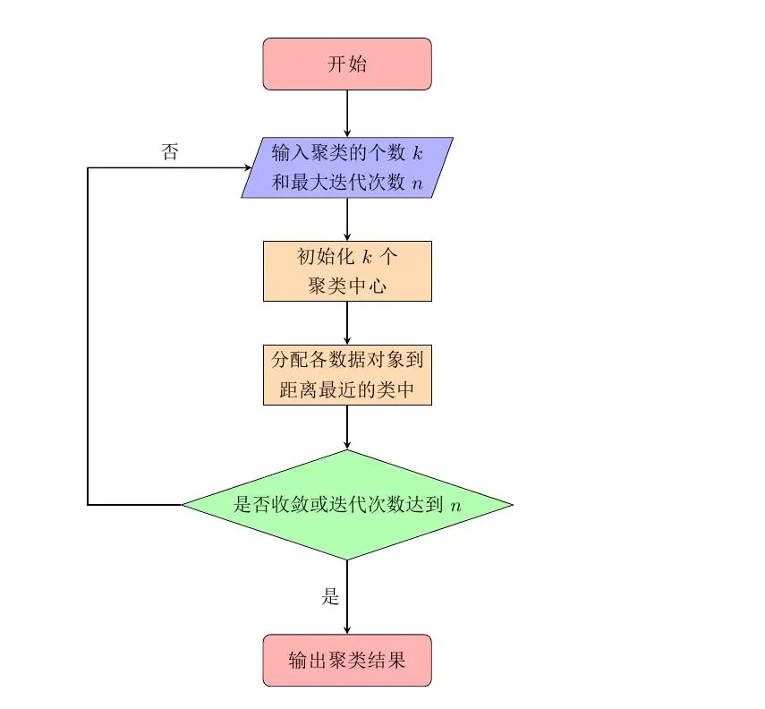
\node (start) [startstop] {开始};
\node (input1) [io,below of=start] {输入聚类的个数 $k$ 和最大迭代次数 $n$ };
\node (process1) [process,below of=input1] {初始化 $k$ 个聚类中心};
\node (process2) [process,below of=process1] {分配各数据对象到距离最近的类中};
\node (decision1) [decision,below of=process2,yshift=-0.5cm] {是否收敛或迭代次数达到 $n$ };
\node (stop) [startstop,below of=decision1,node distance=3cm] {输出聚类结果};
\node(point1)[point,left of=input1,node distance=5cm]{};
\draw [arrow] (start) -- (input1);
\draw [arrow] (input1) -- (process1);
\draw [arrow] (process1) -- (process2);
\draw [arrow] (process2) -- (decision1);
\draw [arrow] (decision1) -- node[anchor=east] {是} (stop);
\draw [straightline] (decision1) -| (point1);
\draw [arrow] (point1) -- node[anchor=south] {否} (input1);
\end{tikzpicture}
\end{document}
# 线粗:
thick:粗
thin:细
# 箭头
->:反向箭头
<-:正向箭头
<->:双向箭头
# 虚线
dashed
# 箭头形状
>=stealth
# name
(decision1):这个节点的name,后面需要用这个name调用这个节点。
# 属性
decision:需要调用的节点的属性
# 位置
below of=process1:定义节点的位置
left of:
right of:
# 偏移,对位置进行微调
yshift:
xshift:
# 属性
[arrow]:需要调用的箭头的属性
(decision1):箭头的其实位置
(process2a):箭头的末端位置
# 线型
--:直线
|-:先竖线后横线
-|:向横线后竖线
# 文字:如果需要在箭头上添加文字
{yes}:需要添加的文字
# 文字的位置,上南下北左东右西(与地图方位不一致)
[anchor=east]:
[anchor=south]:
[anchor=west]:
[anchor=north]:
[anchor=center]:
\documentclass[11pt]{article}
\usepackage{tikz}
\usetikzlibrary{shadows,arrows,positioning,shapes.geometric} % Define the layers to draw the diagram
\pgfdeclarelayer{background}
\pgfdeclarelayer{foreground}
\pgfsetlayers{background,main,foreground}
\tikzstyle{TDK} = [rectangle, rounded corners, minimum width=3cm, minimum height=1cm, text centered, text width=4cm, draw=black, fill=red!30, drop shadow]
\tikzstyle{CFX} = [rectangle, rounded corners, minimum width=3cm, minimum height=1cm, text centered, text width=4cm, draw=black, fill=blue!30, drop shadow]
\tikzstyle{Matlab} = [trapezium, trapezium left angle=70, trapezium right angle=110, minimum width=3cm, minimum height=1cm, text centered, text width=4cm, draw=black, fill=orange!30, drop shadow]
\tikzstyle{arrow} = [thick, ->, >=stealth]
\tikzstyle{texto} = [above, text width=6em, text centered]
\tikzstyle{linepart} = [draw, thick, color=black!50, -latex', dashed] \tikzstyle{line} = [draw, thick, color=black!50, -latex']
% Define distances for bordering \newcommand{\blockdist}{1.3} \newcommand{\edgedist}{1.5}
\newcommand{\etape}[2]{node (p#1) [etape] {#2}}
\newcommand{\matlab}[2]{node (p#1) [Matlab] {#2}}
\newcommand{\tdk}[2]{node (p#1) [TDK] {#2}}
\newcommand{\cfx}[2]{node (p#1) [CFX] {#2}}
% Draw background
\newcommand{\background}[5]{%
\begin{pgfonlayer}{background} % Left-top corner of the background rectangle
\path (#1.west |- #2.north)+(-0.5,0.25) node (a1) {};
% Right-bottom corner of the background rectanle
\path (#3.east |- #4.south)+(+0.5,-0.25) node (a2) {}; % Draw the background
\path[fill=yellow!20,rounded corners, draw=black!50, dashed] (a1) rectangle (a2);
\path (#3.east |- #2.north)+(0,0.25)--(#1.west |- #2.north) node[midway] (#5-n) {};
\path (#3.east |- #2.south)+(0,-0.35)--(#1.west |- #2.south) node[midway] (#5-s) {};
\path (#3.east |- #2.north)+(0.7,0)--(#3.east |- #4.south) node[midway] (#5-w) {};
\path (a1.east |- a1.south)+(1.3,-1.3) node (u1)[texto] {\textit{#5}}; \end{pgfonlayer}}
\newcommand{\transreceptor}[3]{%
\path [linepart] (#1.east) -- node [above] {\scriptsize #2} (#3);}
\begin{document}
\noindent
\begin{tikzpicture}[node distance=2cm,x=0.675cm,y=0.6cm]
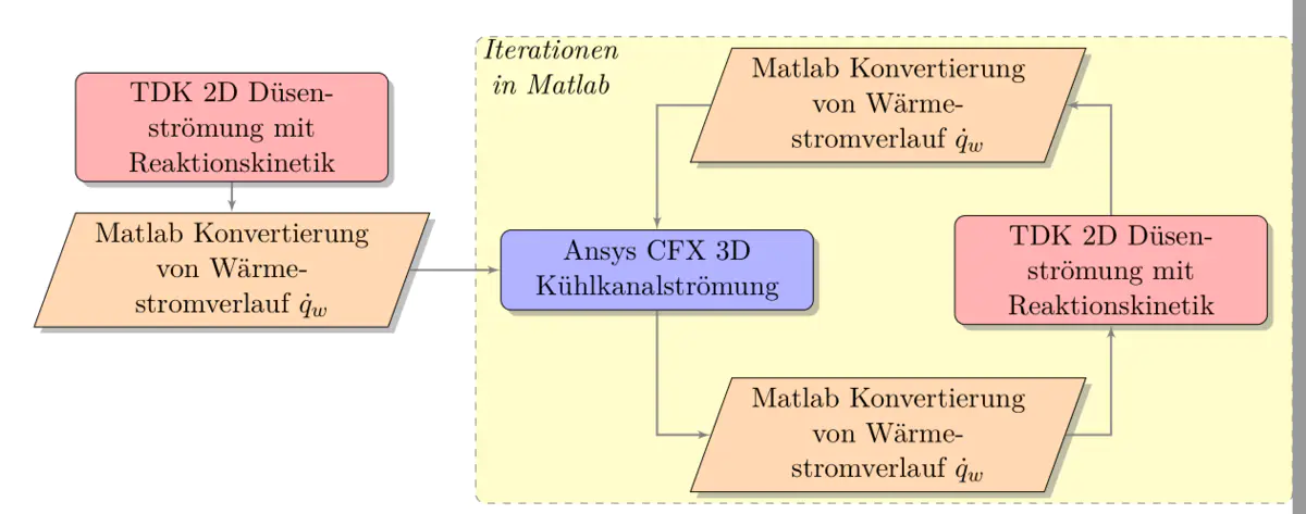
\path \tdk{1}{TDK 2D Düsenströmung mit Reaktionskinetik};
\path (p1.south)+(0.0,-2.0)\matlab{2}{Matlab Konvertierung von Wärmestromverlauf $\dot{q}_w$};
\path (p2.east)+(5.0,0.0) \cfx{3}{Ansys CFX 3D Kühlkanalströmung};
\path (p3.east)+(6.0,0.0) \tdk{4}{TDK 2D Düsenströmung mit Reaktionskinetik};
\path (p4.north)+(-4.5,2.5) \matlab{5}{Matlab Konvertierung von Wärmestromverlauf $\dot{q}_w$};
\path (p4.south)+(-4.5,-2.5) \matlab{6}{Matlab Konvertierung von Wärmestromverlauf $\dot{q}_w$};
\path [line] (p1.south) -- node [above] {} (p2);
\path [line] (p2.east) -- node [above] {} (p3); \path [line] (p3.south) |- node [above] {} (p6);
\path [line] (p4.north) |- node [below] {} (p5);
\path [line] (p6.east) -| node [above] {} (p4);
\path [line] (p5.west) -| node [above] {} (p3);
\background{p3}{p5}{p4}{p6}{Iterationen in Matlab}
\end{tikzpicture}
\end{document}
\documentclass[11pt]{article}
\usepackage{tikz}
\usetikzlibrary{shadows,arrows,positioning}
% Define the layers to draw the diagram
\pgfdeclarelayer{background}
\pgfdeclarelayer{foreground}
\pgfsetlayers{background,main,foreground}
% Define block styles
\tikzstyle{materia}=[draw, fill=blue!20, text width=6.0em, text centered,
minimum height=1.5em,drop shadow]
\tikzstyle{etape} = [materia, text width=8em, minimum width=10em,
minimum height=3em, rounded corners, drop shadow]
\tikzstyle{texto} = [above, text width=6em, text centered]
\tikzstyle{linepart} = [draw, thick, color=black!50, -latex', dashed]
\tikzstyle{line} = [draw, thick, color=black!50, -latex']
\tikzstyle{ur}=[draw, text centered, minimum height=0.01em]
% Define distances for bordering
\newcommand{\blockdist}{1.3}
\newcommand{\edgedist}{1.5}
\newcommand{\etape}[2]{node (p#1) [etape]
{#2}}
% Draw background
\newcommand{\background}[5]{%
\begin{pgfonlayer}{background}
% Left-top corner of the background rectangle
\path (#1.west |- #2.north)+(-0.5,0.25) node (a1) {};
% Right-bottom corner of the background rectanle
\path (#3.east |- #4.south)+(+0.5,-0.25) node (a2) {};
% Draw the background
\path[fill=yellow!20,rounded corners, draw=black!50, dashed]
(a1) rectangle (a2);
\path (#3.east |- #2.north)+(0,0.25)--(#1.west |- #2.north) node[midway] (#5-n) {};
\path (#3.east |- #2.south)+(0,-0.35)--(#1.west |- #2.south) node[midway] (#5-s) {};
\path (#3.east |- #2.north)+(0.7,0)--(#3.east |- #4.south) node[midway] (#5-w) {};
\end{pgfonlayer}}
\newcommand{\transreceptor}[3]{%
\path [linepart] (#1.east) -- node [above]
{\scriptsize #2} (#3);}
\begin{document}
\begin{tikzpicture}[scale=0.7,transform shape]
% Draw diagram elements
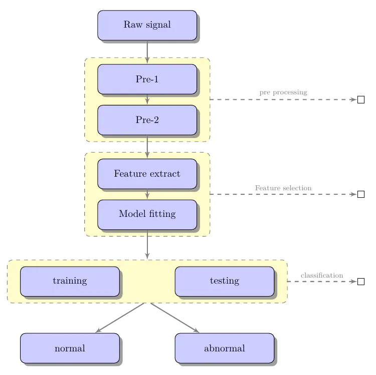
\path \etape{1}{Raw signal};
\path (p1.south)+(0.0,-1.5) \etape{2}{Pre-1};
\path (p2.south)+(0.0,-1.0) \etape{3}{Pre-2};
\path (p3.south)+(0.0,-1.5) \etape{4}{Feature extract};
\path (p4.south)+(0.0,-1.0) \etape{5}{Model fitting};
\path (p5.south)+(-3.0,-2.0) \etape{6}{training};
\path (p5.south)+(3.0,-2.0) \etape{7}{testing};
\node [below=of p5] (p6-7) {};
\path (p6.south)+(0.0,-2.0) \etape{8}{normal};
\path (p7.south)+(0.0,-2.0) \etape{9}{abnormal};
\node [below=of p6-7] (p8-9) {};
% Draw arrows between elements
\path [line] (p1.south) -- node [above] {} (p2);
\path [line] (p2.south) -- node [above] {} (p3);
\path [line] (p3.south) -- node [above] {} (p4);
\path [line] (p4.south) -- node [above] {} (p5);
\background{p2}{p2}{p3}{p3}{bk1}
\background{p4}{p4}{p5}{p5}{bk2}
\background{p6}{p6}{p7}{p7}{bk3}
\path [line] (p5.south) -- node [above] {} (bk3-n);
\path [line] (bk3-s) -- node [above] {} (p8);
\path [line] (bk3-s) -- node [above] {} (p9);
\path (bk1-w)+(+6.0,0) node (ur1)[ur] {};
\path (bk2-w)+(+6.0,0) node (ur2)[ur] {};
\path (bk3-w)+(+3.0,0) node (ur3)[ur] {};
\transreceptor{bk1-w}{pre processing}{ur1};
\transreceptor{bk2-w}{Feature selection}{ur2};
\transreceptor{bk3-w}{classification}{ur3};
\end{tikzpicture}
\end{document}
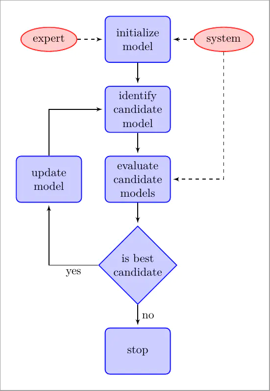
\documentclass[border=10pt]{standalone}
\usepackage{tikz}
\usetikzlibrary{shapes.geometric}
\usetikzlibrary{arrows.meta,arrows}
\begin{document}
\begin{tikzpicture}
[auto,
decision/.style={diamond, draw=blue, thick, fill=blue!20,
    text width=4.5em,align=flush center,
    inner sep=1pt},
block/.style ={rectangle, draw=blue, thick, fill=blue!20,
    text width=5em,align=center, rounded corners,
    minimum height=4em},
line/.style ={draw, thick, -latex',shorten >=2pt},
cloud/.style ={draw=red, thick, ellipse,fill=red!20,
    minimum height=2em}]
\matrix [column sep=5mm,row sep=7mm]
{
    % row 1
    \node [cloud] (expert) {expert}; &
    \node [block] (init) {initialize model}; &
    \node [cloud] (system) {system}; \\
    % row 2
    & \node [block] (identify) {identify candidate model}; & \\
    % row 3
    \node [block] (update) {update model}; &
    \node [block] (evaluate) {evaluate candidate models}; & \\
    % row 4
    & \node [decision] (decide) {is best candidate}; & \\
    % row 5
    & \node [block] (stop) {stop}; & \\
};
\begin{scope}[every path/.style=line]
\path (init) -- (identify);
\path (identify) -- (evaluate);
\path (evaluate) -- (decide);
\path (update) |- (identify);
\path (decide) -| node [near start] {yes} (update);
\path (decide) -- node [midway] {no} (stop);
\path [dashed] (expert) -- (init);
\path [dashed] (system) -- (init);
\path [dashed] (system) |- (evaluate);
\end{scope}
\end{tikzpicture}
\end{document}
\documentclass{article}
\usepackage{pgf}
\usepackage{tikz}
\usetikzlibrary{arrows, decorations.pathmorphing, backgrounds, positioning, fit, petri, automata}
\definecolor{yellow1}{rgb}{1,0.8,0.2}
%opening
\begin{document}
\begin{tikzpicture}[->,>=stealth',shorten >=1pt,auto,node distance=2.8cm,
semithick]
\tikzstyle{every state}=[fill=yellow1,draw=none,text=black]
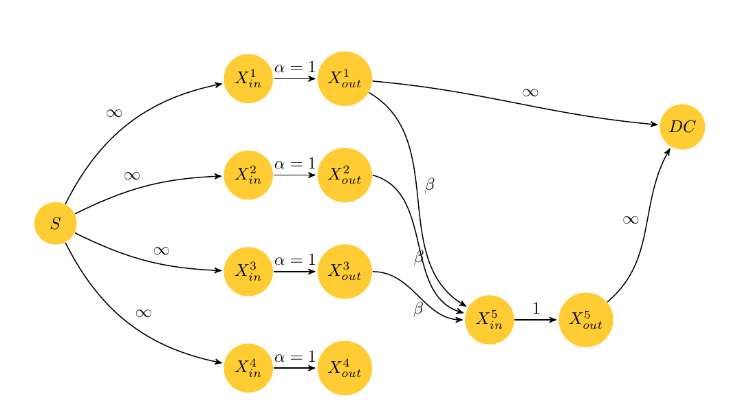
\node[state] (S) at (-6, 0) {$S$};
\node[state] (xin1) at (-2, 3) {$X^1_{in}$};
\node[state] (xin2) at (-2, 1) {$X^2_{in}$};
\node[state] (xin3) at (-2, -1) {$X^3_{in}$};
\node[state] (xin4) at (-2, -3) {$X^4_{in}$};
\node[state] (xout1) at (0, 3) {$X^1_{out}$};
\node[state] (xout2) at (0, 1) {$X^2_{out}$};
\node[state] (xout3) at (0, -1) {$X^3_{out}$};
\node[state] (xout4) at (0, -3) {$X^4_{out}$};
\node[state] (xin5) at (3, -2) {$X^5_{in}$};
\node[state] (xout5) at (5, -2) {$X^5_{out}$};
\node[state] (DC) at (7, 2) {$DC$};
\path (S) edge[bend left=26] node {$\infty$} (xin1)
edge[bend left=12] node {$\infty$} (xin2)
edge[bend right=12] node {$\infty$} (xin3)
edge[bend right=26] node {$\infty$} (xin4)
(xin1) edge node {$\alpha=1$} (xout1)
(xin2) edge node {$\alpha=1$} (xout2)
(xin3) edge node {$\alpha=1$} (xout3)
(xin4) edge node {$\alpha=1$} (xout4)
(xin5) edge node {$1$} (xout5);
\draw[->] (xout1) to[out=-30,in=150] node {$\beta$} (xin5);
\draw[->] (xout2.east) to[out=-15,in=165] node [below] {$\beta$} (xin5);
\draw[->] (xout3.east) to[out=0,in=180] node [below] {$\beta$} (xin5.west);
\draw[->] (xout1) to[out=-5,in=175] node {$\infty$} (DC);
\draw[->] (xout5) to[out=40, in=-120] node {$\infty$} (DC);
\end{tikzpicture}
\end{document}