最小二乘法应用：用直线或曲线模型拟合散点

记录下用最小二乘法拟合线性模型的代码实现：

1、应用正规方程（Normal Equation)求解最小二乘法举例：

最简单的y关于x的线性方程\(y=\beta_0+\beta_1x\)

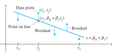
预测值和观察值：

 

 写成矩阵形式：

\(X\beta=y\)，其中\(X=\begin{bmatrix} 1& x_1\\ 1& x_2\\ ...&...\\ 1& x_n\\ \end{bmatrix}\) ， \(\beta=\begin{bmatrix} \beta_0\\ \beta_1\\ \end{bmatrix}\) ， \(y=\begin{bmatrix} y_1\\ y_2\\ ...\\ y_n\\ \end{bmatrix}\)

最小二乘法的解\(\beta\)可以通过解正规方程获得： \(X^TX\beta=X^Ty\)

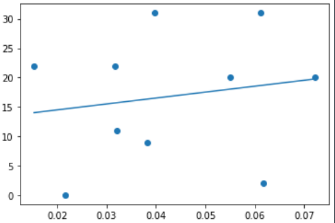
python代码实现如下：

import numpy as np
from numpy.linalg import inv


x=[0.015348106072082663,0.021715879765738008,0.0316253067336889,
   0.03212431406271639,0.03828189026158509,0.03965578961513808,
   0.05502733389871053,0.06116957740576664,0.06170785924013203,
   0.07206404835977503]
y=[22, 0, 22, 11, 9, 31, 20, 31, 2, 20]


def plotLinearRegression1():
    X = np.array(x).reshape(len(x),1)
    reg=linear_model.LinearRegression(fit_intercept=True,normalize=False)
    reg.fit(X,y)
    k=reg.coef_#获取斜率w1,w2,w3,...,wn
    b=reg.intercept_#获取截距w0
    #x0=np.arange(0,10,0.2)
    x0 = np.array(x).reshape(len(x),)
    y0=k*x0+b
    plt.scatter(x,y)
    plt.plot(x0, y0)
    print('k',k);
    print('b',b)
  
      
'''
用least squares
'''
def plotLinearRegression2():
    X = np.vstack([np.ones((1,len(x))),x]).T
    print('X:\n',X)
    Xt = X.T
    Z = Xt.dot(X)
    invZ = inv(Z)
    print('invZ:\n',invZ)
    
    W = (invZ.dot(Xt)).dot(y)
    print('W:\n',W)
    
    #plot
    plt.scatter(x,y)
    x0 = np.array(x).reshape(len(x),)
   # x0=np.arange(0,10,0.2)
    plt.plot(x0, W[1]*x0+W[0])
    
    
def plotLinearRegression3():
    A = np.vstack([x, np.ones(len(x))]).T
    print('A:\n',A)
    m, c = np.linalg.lstsq(A, y, rcond=None)[0]
    print('m: ',m,'  c:',c)
   
    x0 = np.array(x).reshape(len(x),)
    plt.plot(x, y, 'o', label='Original data', markersize=10)
    plt.plot(x0, m*x0 + c, 'r', label='Fitted line')
    plt.legend()
    plt.show()  
    
        
if __name__ == '__main__':
    plotLinearRegression2()

 

 

2、记录用最小二乘法拟合曲线模型

题目：（来源于书本《Linear Algebra And Its Applications Fifth Edition - David C.Lay ·  Steven R.Lay · Judi J. McDonald》）

 

 

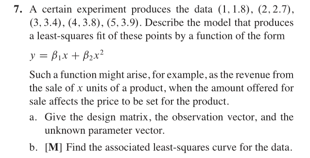
 解：

\(\bold{y}=\bold{x}\beta+\boldsymbol{\varepsilon}\)，\(\bold{y}\) = \(\begin{bmatrix}
1.8
\\ 2.7
\\ 3.4
\\ 3.8
\\3.9
\end{bmatrix}\)，\(\bold{x} = \begin{bmatrix}
1 & 1\\
2 & 4\\
3 & 9\\
4 & 16\\
5 & 25
\end{bmatrix}\)， \(\boldsymbol{\beta } = \begin{bmatrix}
\beta _{1}\\
\beta _{2}
\end{bmatrix}\)， \(\boldsymbol{\varepsilon } = \begin{bmatrix}
\varepsilon _{1}\\
\varepsilon _{2}\\
\varepsilon _{3}\\
\varepsilon _{4}\\
\varepsilon _{5}
\end{bmatrix}\)

 由\(\bold{x}^T\bold{x}\boldsymbol{\beta}=\bold{x}^T\bold{y}\) 得 \(\boldsymbol{\beta} = (\bold{x^{T}x})^{-1}\bold{x^{T}}\bold{y}\)

octave计算结果如下：

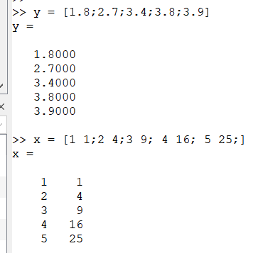
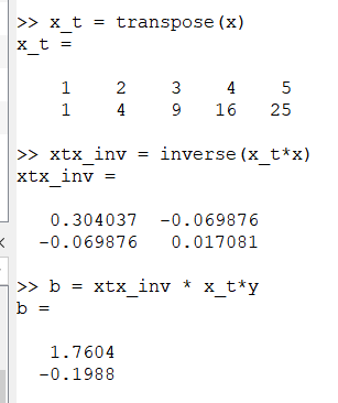
得\(\beta_{1} = 1.76，\beta_{2} = -0.20\)

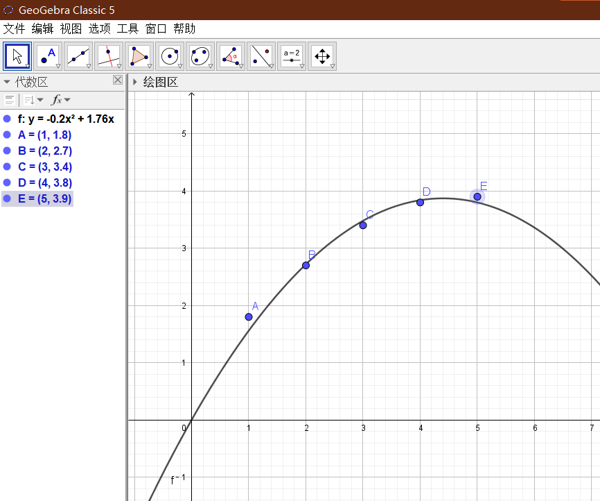
曲线方程为：\(y = 1.76x - 0.20x^2\)

拟合效果如下图：