神经网络和深度学习-week3编程题(具有一个隐藏层的平面数据分类)

建立神经网络的步骤:
1.定义模型结构(eg输入特征的数量)
2.初始化模型的参数
3.循环求解最终参数:
- 计算当前损失(正向传播)
- 计算当前梯度(反向传播)
- 更新参数(梯度下降)
4.预测
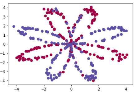
提前加载和查看数据
 1 import numpy as np
 2 import matplotlib.pyplot as plt
 3 from testCases import *
 4 import sklearn
 5 import sklearn.datasets
 6 import sklearn.linear_model
 7 from planar_utils import plot_decision_boundary, sigmoid, load_planar_dataset, load_extra_datasets
 8
 9
10 np.random.seed(1) # set a seed so that the results are consistent
11 X, Y = load_planar_dataset()     #X(2,400)数据点数值  Y(1,400)对应X的标签0或1
12 m=X.shape[1]                     #400个数据
13
14 # Visualize the data:
15 plt.scatter(X[0, :], X[1, :], c=np.squeeze(Y), s=40, cmap = plt.cm.Spectral)
定义神经网络结构
输入:X,Y是数据集和标签
返回:n_x,n_h,n_y分别表示输入层、隐藏层(规定为4)和输出层的数量
1 def layer_sizes(X, Y):
2
3     n_x=X.shape[0]
4     n_h=4
5     n_y=Y.shape[0]
6
7     return (n_x, n_h, n_y)
初始化模型参数
输入:n_x,n_h,n_y分别表示输入层、隐藏层(规定为4)和输出层的数量
返回:参数(W1,b1,W2,b2)
 1 def initialize_parameters(n_x, n_h, n_y):
 2
 3     np.random.seed(2)
 4
 5     ### START CODE HERE ### (≈ 4 lines of code)
 6     W1=np.random.randn(n_h, n_x)*0.01
 7     W2=np.random.randn(n_y,n_h)*0.01
 8
 9     b1=np.zeros((n_h,1))
10     b2=np.zeros((n_y,1))
11     ### END CODE HERE ###
12
13     assert (W1.shape == (n_h, n_x))
14     assert (b1.shape == (n_h, 1))
15     assert (W2.shape == (n_y, n_h))
16     assert (b2.shape == (n_y, 1))
17
18     parameters = {"W1": W1,
19                   "b1": b1,
20                   "W2": W2,
21                   "b2": b2}
22
23     return parameters
Forward propagation 前向传播

输入:数据集X,初始化得到的参数parameters(包含W1,b1,W2,b2)
返回:包含Z1,A1,Z2,A2的cache值(用来作为反向传输的输入)
 1 def forward_propagation(X, parameters):
 2
 3     # Retrieve each parameter from the dictionary "parameters"
 4     ### START CODE HERE ### (≈ 4 lines of code)
 5     W1=parameters['W1']
 6     b1=parameters['b1']
 7     W2=parameters['W2']
 8     b2=parameters['b2']
 9     ### END CODE HERE ###
10
11     # Implement Forward Propagation to calculate A2 (probabilities)
12     ### START CODE HERE ### (≈ 4 lines of code)
13     Z1=np.dot(W1,X)+b1
14     A1=np.tanh(Z1)
15
16     Z2=np.dot(W2,A1)+b2
17     A2=sigmoid(Z2)
18     ### END CODE HERE ###
19
20     assert(A2.shape == (1, X.shape[1]))
21
22     cache = {"Z1": Z1,
23              "A1": A1,
24              "Z2": Z2,
25              "A2": A2}
26
27     return A2, cache
计算损失
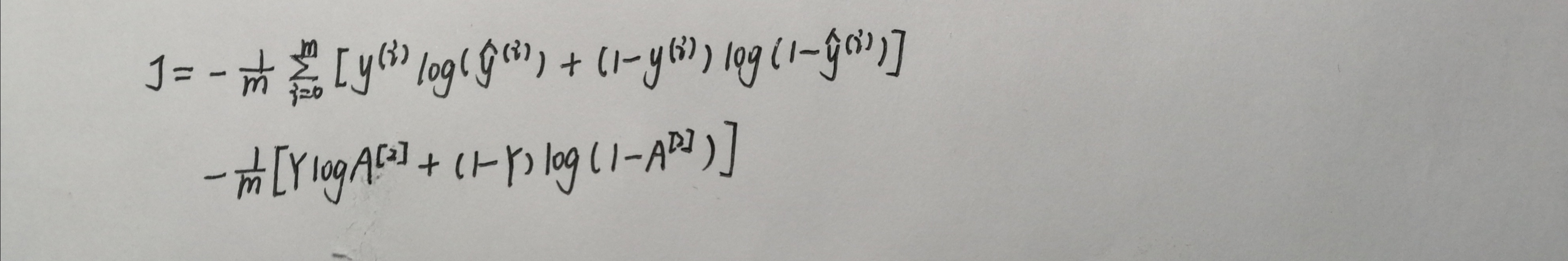
输入:A2表示二次激活后的数值,Y表示数据标签(1,400),参数parameters(包含W1,b1,W2,b2)
返回:计算得到的成本
 1 def compute_cost(A2, Y, parameters):
 2
 3     m = Y.shape[1] # number of example
 4
 5     # Retrieve W1 and W2 from parameters
 6     ### START CODE HERE ### (≈ 2 lines of code)
 7     W1=parameters['W1']
 8     W2=parameters['W2']
 9     ### END CODE HERE ###
10
11     # Compute the cross-entropy cost
12     ### START CODE HERE ### (≈ 2 lines of code)
13     logprobs = np.multiply(np.log(A2),Y) + np.multiply((1 - Y), np.log(1 - A2))
14     cost = - np.sum(logprobs) / m
15     ### END CODE HERE ###
16
17     cost = float(np.squeeze(cost))     # makes sure cost is the dimension we expect.
18                                        # E.g., turns [[17]] into 17
19     assert(isinstance(cost, float))
20
21     return cost
Backward propagation反向传播
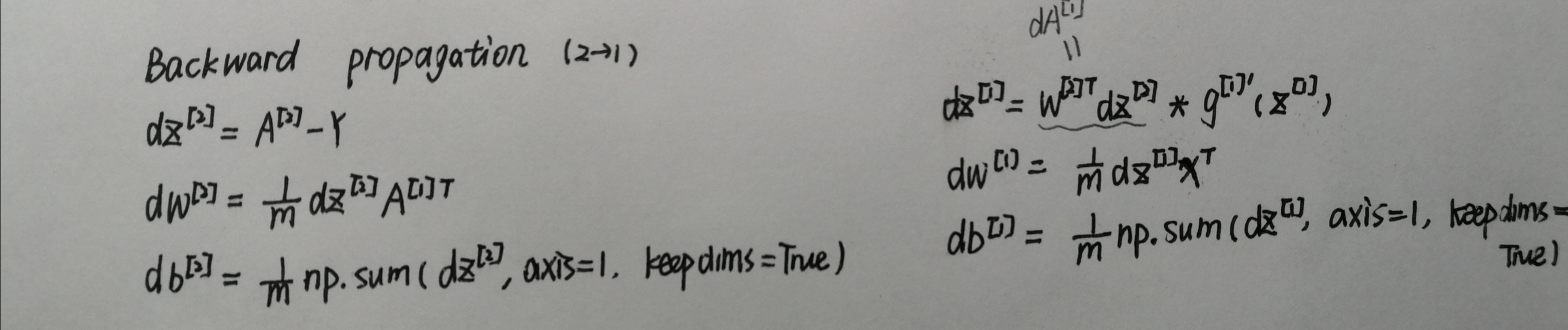
输入:参数parameters(包含W1,b1,W2,b2),参数cache(包含Z1,A1,Z2,A2),X表示数据集,Y表示数据标签
返回:包含dW1,db1,dW2,db2的grads
 1 def backward_propagation(parameters, cache, X, Y):
 2
 3     m = X.shape[1]
 4
 5     # First, retrieve W1 and W2 from the dictionary "parameters".
 6     ### START CODE HERE ### (≈ 2 lines of code)
 7     W1=parameters['W1']
 8     W2=parameters['W2']
 9     ### END CODE HERE ###
10
11     # Retrieve also A1 and A2 from dictionary "cache".
12     ### START CODE HERE ### (≈ 2 lines of code)
13     A1=cache['A1']
14     A2=cache['A2']
15     ### END CODE HERE ###
16
17     # Backward propagation: calculate dW1, db1, dW2, db2.
18     ### START CODE HERE ### (≈ 6 lines of code, corresponding to 6 equations on slide above)
19     dZ2=A2-Y
20     dW2=np.dot(dZ2,A1.T)/m
21     db2=np.sum(dZ2,axis=1,keepdims=True)/m
22
23     dZ1=np.multiply(np.dot(W2.T, dz2), 1 - np.power(A1, 2))
24     dW1=np.dot(dZ1,X.T)/m
25     db1=np.sum(dZ1,axis=1,keepdims=True)/m
26     ### END CODE HERE ###
27
28     grads = {"dW1": dW1,
29              "db1": db1,
30              "dW2": dW2,
31              "db2": db2}
32
33     return grads
更新参数
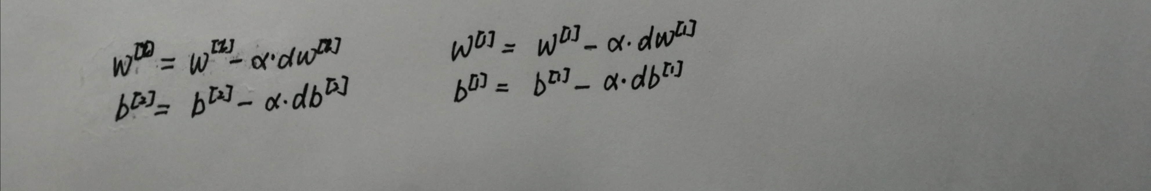
输入:参数parameters(包含W1,b1,W2,b2),参数grads(包含dW1,db1,dW2,db2),学习速率learning_rate
返回:参数parameters(包含W1,b1,W2,b2)
 1 def update_parameters(parameters, grads, learning_rate=1.2):
 2
 3     # Retrieve each parameter from the dictionary "parameters"
 4     ### START CODE HERE ### (≈ 4 lines of code)
 5     W1=parameters['W1']
 6     b1=parameters['b1']
 7     W2=parameters['W2']
 8     b2=parameters['b2']
 9     ### END CODE HERE ###
10
11     # Retrieve each gradient from the dictionary "grads"
12     ### START CODE HERE ### (≈ 4 lines of code)
13     dW1=grads['dW1']
14     db1=grads['db1']
15     dW2=grads['dW2']
16     db2=grads['db2']
17     ## END CODE HERE ###
18
19     # Update rule for each parameter
20     ### START CODE HERE ### (≈ 4 lines of code)
21     W1=W1-learning_rate*dW1
22     W2=W2-learning_rate*dW2
23     b1=b1-learning_rate*db1
24     b2=b2-learning_rate*db2
25
26     ### END CODE HERE ###
27
28     parameters = {"W1": W1,
29                   "b1": b1,
30                   "W2": W2,
31                   "b2": b2}
32
33     return parameters
封装函数
输入:X表示数据集,Y表示数据标签,n_h表示隐藏层层数,num_iterations表示迭代次数
返回:最终参数parameters(包含W1,b1,W2,b2)
def nn_model(X, Y, n_h, num_iterations=10000, print_cost=False):

    np.random.seed(3)
    n_x = layer_sizes(X, Y)[0]
    n_y = layer_sizes(X, Y)[2]

    # Initialize parameters, then retrieve W1, b1, W2, b2. Inputs: "n_x, n_h, n_y". Outputs = "W1, b1, W2, b2, parameters".
    ### START CODE HERE ### (≈ 5 lines of code)
    parameters=initialize_parameters(n_x, n_h, n_y)
    W1=parameters['W1']
    b1=parameters['b1']
    W2=parameters['W2']
    b2=parameters['b2']
    ### END CODE HERE ###

    # Loop (gradient descent)
    for i in range(0, num_iterations):

        ### START CODE HERE ### (≈ 4 lines of code)
        # Forward propagation. Inputs: "X, parameters". Outputs: "A2, cache".
        A2,cache=forward_propagation(X, parameters)

        # Cost function. Inputs: "A2, Y, parameters". Outputs: "cost".
        cost=compute_cost(A2, Y, parameters)

        # Backpropagation. Inputs: "parameters, cache, X, Y". Outputs: "grads".
        grads=backward_propagation(parameters, cache, X, Y)

        # Gradient descent parameter update. Inputs: "parameters, grads". Outputs: "parameters".
        parameters=update_parameters(parameters, grads)
        ### END CODE HERE ###

        # Print the cost every 1000 iterations
        if print_cost and i % 1000 == 0:
            print ("Cost after iteration %i: %f" % (i, cost))

    return parameters
预测
输入:从nn_model函数返回的参数parameters(包含W1,b1,W2,b2),X为数据集
返回:仅含有0和1的数组
1 def predict(parameters, X):
2
3     # Computes probabilities using forward propagation, and classifies to 0/1 using 0.5 as the threshold.
4     ### START CODE HERE ### (≈ 2 lines of code)
5     A2 , cache = forward_propagation(X,parameters)
6     predictions = np.round(A2)
7     ### END CODE HERE ###
8
9     return predictions
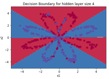
1 parameters = nn_model(X, Y, n_h = 4, num_iterations=10000, print_cost=True)
2
3 #绘制边界
4 plot_decision_boundary(lambda x: predict(parameters, x.T), X, Y)
5 plt.title("Decision Boundary for hidden layer size " + str(4))
6
7 predictions = predict(parameters, X)8 print ('准确率: %d' % float((np.dot(Y, predictions.T) + np.dot(1 - Y, 1 - predictions.T)) / float(Y.size) * 100) + '%')
运行结果:
不同隐藏层节点数量的预测准确率
 1 plt.figure(figsize=(16, 32))
 2 hidden_layer_sizes = [1, 2, 3, 4, 5, 20, 50]
 3 for i, n_h in enumerate(hidden_layer_sizes):
 4     plt.subplot(5, 2, i + 1)
 5     plt.title('Hidden Layer of size %d' % n_h)
 6     parameters = nn_model(X, Y, n_h, num_iterations=5000)
 7     plot_decision_boundary(lambda x: predict(parameters, x.T), X, Y)
 8     predictions = predict(parameters, X)
 9     accuracy = float((np.dot(Y, predictions.T) + np.dot(1 - Y, 1 - predictions.T)) / float(Y.size) * 100)
10     print ("Accuracy for {} hidden units: {} %".format(n_h, accuracy))
