tensorflow神经网络拟合非线性函数与操作指南
本实验通过建立一个含有两个隐含层的BP神经网络,拟合具有二次函数非线性关系的方程,并通过可视化展现学习到的拟合曲线,同时随机给定输入值,输出预测值,最后给出一些关键的提示。
源代码如下:
# -*- coding: utf-8 -*-
import tensorflow as tf
import numpy as np
import matplotlib.pyplot as plt

plotdata = { "batchsize":[], "loss":[] }
def moving_average(a, w=11):
    if len(a) < w:
        return a[:]
    return [val if idx < w else sum(a[(idx-w):idx])/w for idx, val in enumerate(a)]

#生成模拟数据,二次函数关系
train_X = np.linspace(-1, 1, 100)[:, np.newaxis]
train_Y = train_X*train_X + 5 * train_X + np.random.randn(*train_X.shape) * 0.3

#子图1显示模拟数据点
plt.figure(12)
plt.subplot(221)
plt.plot(train_X, train_Y, 'ro', label='Original data')
plt.legend()

# 创建模型
# 占位符
X = tf.placeholder("float",[None,1])
Y = tf.placeholder("float",[None,1])
# 模型参数
W1 = tf.Variable(tf.random_normal([1,10]), name="weight1")
b1 = tf.Variable(tf.zeros([1,10]), name="bias1")
W2 = tf.Variable(tf.random_normal([10,6]), name="weight2")
b2 = tf.Variable(tf.zeros([1,6]), name="bias2")
W3 = tf.Variable(tf.random_normal([6,1]), name="weight3")
b3 = tf.Variable(tf.zeros([1]), name="bias3")

# 前向结构
z1 = tf.matmul(X, W1) + b1
z2 = tf.nn.relu(z1)
z3 = tf.matmul(z2, W2) + b2
z4 = tf.nn.relu(z3)
z5 = tf.matmul(z4, W3) + b3

#反向优化
cost =tf.reduce_mean( tf.square(Y - z5))
learning_rate = 0.01
optimizer = tf.train.GradientDescentOptimizer(learning_rate).minimize(cost) #Gradient descent

# 初始化变量
init = tf.global_variables_initializer()
# 训练参数
training_epochs = 5000
display_step = 2

# 启动session
with tf.Session() as sess:
    sess.run(init)
    for epoch in range(training_epochs+1):
        sess.run(optimizer, feed_dict={X: train_X, Y: train_Y})

        #显示训练中的详细信息
        if epoch % display_step == 0:
            loss = sess.run(cost, feed_dict={X: train_X, Y:train_Y})
            print ("Epoch:", epoch, "cost=", loss)
            if not (loss == "NA" ):
                plotdata["batchsize"].append(epoch)
                plotdata["loss"].append(loss)
    print (" Finish")

    #图形显示
    plt.subplot(222)
    plt.plot(train_X, train_Y, 'ro', label='Original data')
    plt.plot(train_X, sess.run(z5, feed_dict={X: train_X}), label='Fitted line')
    plt.legend()
    plotdata["avgloss"] = moving_average(plotdata["loss"])

    plt.subplot(212)
    plt.plot(plotdata["batchsize"], plotdata["avgloss"], 'b--')
    plt.xlabel('Minibatch number')
    plt.ylabel('Loss')
    plt.title('Minibatch run vs Training loss')
    plt.show()
    #预测结果
    a=[[0.2],[0.3]]
    print ("x=[[0.2],[0.3]],z5=", sess.run(z5, feed_dict={X: a}))
运行结果如下:
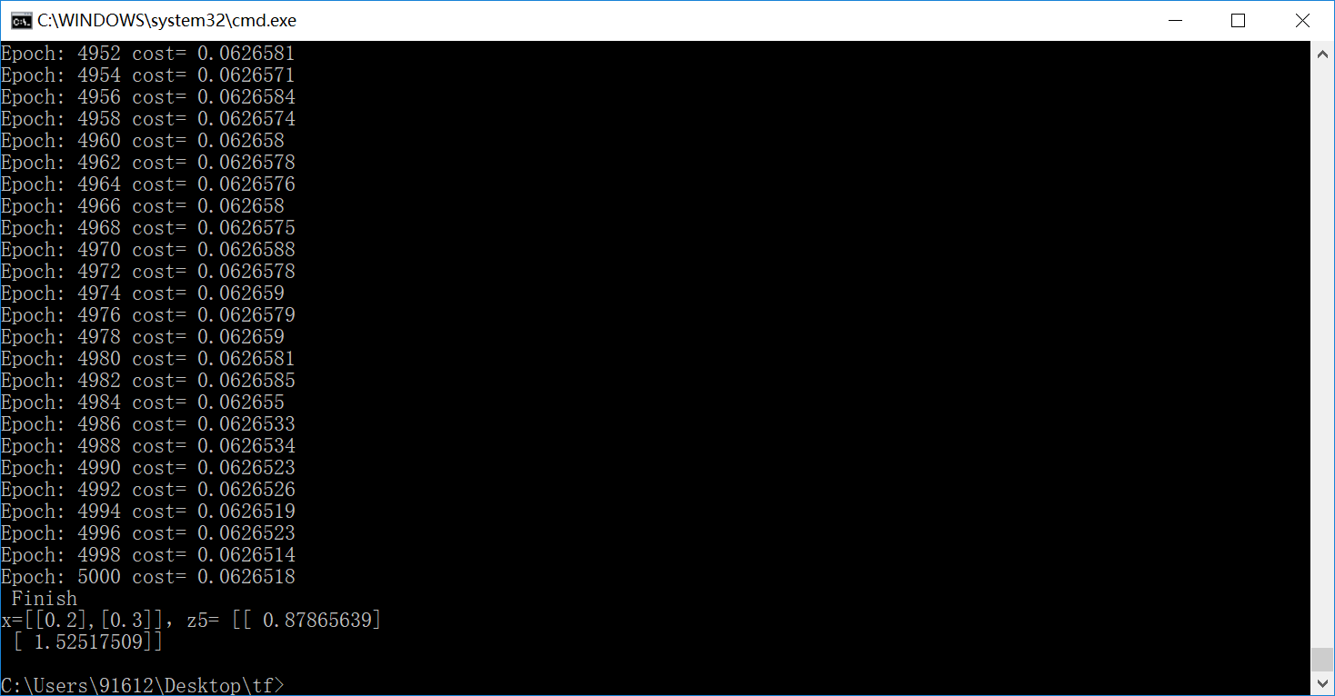
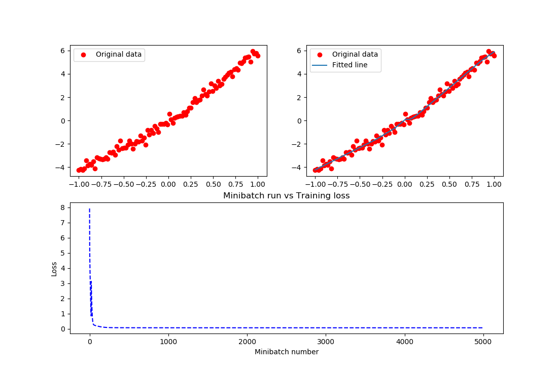
结果实在是太棒了,把这个关系拟合的非常好。在上述的例子中,需要进一步说明如下内容:
- 输入节点可以通过字典类型定义,而后通过字典的方法访问
input = {
    'X': tf.placeholder("float",[None,1]),
    'Y': tf.placeholder("float",[None,1])
}
sess.run(optimizer, feed_dict={input['X']: train_X, input['Y']: train_Y})
直接定义输入节点的方法是不推荐使用的。
- 变量也可以通过字典类型定义,例如上述代码可以改为:
parameter = {
    'W1': tf.Variable(tf.random_normal([1,10]), name="weight1"),
    'b1': tf.Variable(tf.zeros([1,10]), name="bias1"),
    'W2': tf.Variable(tf.random_normal([10,6]), name="weight2"),
    'b2': tf.Variable(tf.zeros([1,6]), name="bias2"),
    'W3': tf.Variable(tf.random_normal([6,1]), name="weight3"),
    'b3': tf.Variable(tf.zeros([1]), name="bias3")
}
z1 = tf.matmul(X, parameter['W1']) +parameter['b1']
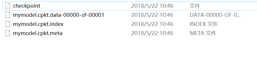
在上述代码中练习保存/载入模型,代码如下:
# -*- coding: utf-8 -*-
import tensorflow as tf
import numpy as np
import matplotlib.pyplot as plt

plotdata = { "batchsize":[], "loss":[] }
def moving_average(a, w=11):
    if len(a) < w:
        return a[:]
    return [val if idx < w else sum(a[(idx-w):idx])/w for idx, val in enumerate(a)]

#生成模拟数据,二次函数关系
train_X = np.linspace(-1, 1, 100)[:, np.newaxis]
train_Y = train_X*train_X + 5 * train_X + np.random.randn(*train_X.shape) * 0.3

#子图1显示模拟数据点
plt.figure(12)
plt.subplot(221)
plt.plot(train_X, train_Y, 'ro', label='Original data')
plt.legend()

# 创建模型
# 字典型占位符
input = {'X':tf.placeholder("float",[None,1]),
         'Y':tf.placeholder("float",[None,1])}
# X = tf.placeholder("float",[None,1])
# Y = tf.placeholder("float",[None,1])
# 模型参数
parameter = {'W1':tf.Variable(tf.random_normal([1,10]), name="weight1"), 'b1':tf.Variable(tf.zeros([1,10]), name="bias1"),
 'W2':tf.Variable(tf.random_normal([10,6]), name="weight2"),'b2':tf.Variable(tf.zeros([1,6]), name="bias2"),
 'W3':tf.Variable(tf.random_normal([6,1]), name="weight3"), 'b3':tf.Variable(tf.zeros([1]), name="bias3")}
# W1 = tf.Variable(tf.random_normal([1,10]), name="weight1")
# b1 = tf.Variable(tf.zeros([1,10]), name="bias1")
# W2 = tf.Variable(tf.random_normal([10,6]), name="weight2")
# b2 = tf.Variable(tf.zeros([1,6]), name="bias2")
# W3 = tf.Variable(tf.random_normal([6,1]), name="weight3")
# b3 = tf.Variable(tf.zeros([1]), name="bias3")

# 前向结构
z1 = tf.matmul(input['X'], parameter['W1']) + parameter['b1']
z2 = tf.nn.relu(z1)
z3 = tf.matmul(z2, parameter['W2']) + parameter['b2']
z4 = tf.nn.relu(z3)
z5 = tf.matmul(z4, parameter['W3']) + parameter['b3']

#反向优化
cost =tf.reduce_mean( tf.square(input['Y'] - z5))
learning_rate = 0.01
optimizer = tf.train.GradientDescentOptimizer(learning_rate).minimize(cost) #Gradient descent

# 初始化变量
init = tf.global_variables_initializer()
# 训练参数
training_epochs = 5000
display_step = 2
# 生成saver
saver = tf.train.Saver()
savedir = "model/"

# 启动session
with tf.Session() as sess:
    sess.run(init)
    for epoch in range(training_epochs+1):
        sess.run(optimizer, feed_dict={input['X']: train_X, input['Y']: train_Y})

        #显示训练中的详细信息
        if epoch % display_step == 0:
            loss = sess.run(cost, feed_dict={input['X']: train_X, input['Y']:train_Y})
            print ("Epoch:", epoch, "cost=", loss)
            if not (loss == "NA" ):
                plotdata["batchsize"].append(epoch)
                plotdata["loss"].append(loss)
    print (" Finish")
    #保存模型
    saver.save(sess, savedir+"mymodel.cpkt")

    #图形显示
    plt.subplot(222)
    plt.plot(train_X, train_Y, 'ro', label='Original data')
    plt.plot(train_X, sess.run(z5, feed_dict={input['X']: train_X}), label='Fitted line')
    plt.legend()
    plotdata["avgloss"] = moving_average(plotdata["loss"])

    plt.subplot(212)
    plt.plot(plotdata["batchsize"], plotdata["avgloss"], 'b--')
    plt.xlabel('Minibatch number')
    plt.ylabel('Loss')
    plt.title('Minibatch run vs Training loss')
    plt.show()

#预测结果
#在另外一个session里面载入保存的模型,再测试
a=[[0.2],[0.3]]
with tf.Session() as sess2:
    #sess2.run(tf.global_variables_initializer())可有可无,因为下面restore会载入参数,相当于本次调用的初始化
    saver.restore(sess2, "model/mymodel.cpkt")
    print ("x=[[0.2],[0.3]],z5=", sess2.run(z5, feed_dict={input['X']: a}))
生成如下目录:
上述代码模型的载入没有利用到检查点文件,显得不够智能,还需用户去查找指定某一模型,那在很多算法项目中是不需要用户去找的,而可以通过检查点找到保存的模型。例如:
# -*- coding: utf-8 -*-
import tensorflow as tf
import numpy as np
import matplotlib.pyplot as plt

plotdata = { "batchsize":[], "loss":[] }
def moving_average(a, w=11):
    if len(a) < w:
        return a[:]
    return [val if idx < w else sum(a[(idx-w):idx])/w for idx, val in enumerate(a)]

#生成模拟数据,二次函数关系
train_X = np.linspace(-1, 1, 100)[:, np.newaxis]
train_Y = train_X*train_X + 5 * train_X + np.random.randn(*train_X.shape) * 0.3

#子图1显示模拟数据点
plt.figure(12)
plt.subplot(221)
plt.plot(train_X, train_Y, 'ro', label='Original data')
plt.legend()

# 创建模型
# 字典型占位符
input = {'X':tf.placeholder("float",[None,1]),
         'Y':tf.placeholder("float",[None,1])}
# X = tf.placeholder("float",[None,1])
# Y = tf.placeholder("float",[None,1])
# 模型参数
parameter = {'W1':tf.Variable(tf.random_normal([1,10]), name="weight1"), 'b1':tf.Variable(tf.zeros([1,10]), name="bias1"),
 'W2':tf.Variable(tf.random_normal([10,6]), name="weight2"),'b2':tf.Variable(tf.zeros([1,6]), name="bias2"),
 'W3':tf.Variable(tf.random_normal([6,1]), name="weight3"), 'b3':tf.Variable(tf.zeros([1]), name="bias3")}
# W1 = tf.Variable(tf.random_normal([1,10]), name="weight1")
# b1 = tf.Variable(tf.zeros([1,10]), name="bias1")
# W2 = tf.Variable(tf.random_normal([10,6]), name="weight2")
# b2 = tf.Variable(tf.zeros([1,6]), name="bias2")
# W3 = tf.Variable(tf.random_normal([6,1]), name="weight3")
# b3 = tf.Variable(tf.zeros([1]), name="bias3")

# 前向结构
z1 = tf.matmul(input['X'], parameter['W1']) + parameter['b1']
z2 = tf.nn.relu(z1)
z3 = tf.matmul(z2, parameter['W2']) + parameter['b2']
z4 = tf.nn.relu(z3)
z5 = tf.matmul(z4, parameter['W3']) + parameter['b3']

#反向优化
cost =tf.reduce_mean( tf.square(input['Y'] - z5))
learning_rate = 0.01
optimizer = tf.train.GradientDescentOptimizer(learning_rate).minimize(cost) #Gradient descent

# 初始化变量
init = tf.global_variables_initializer()
# 训练参数
training_epochs = 5000
display_step = 2
# 生成saver
saver = tf.train.Saver(max_to_keep=1)
savedir = "model/"

# 启动session
with tf.Session() as sess:
    sess.run(init)
    for epoch in range(training_epochs+1):
        sess.run(optimizer, feed_dict={input['X']: train_X, input['Y']: train_Y})
        saver.save(sess, savedir+"mymodel.cpkt",global_step=epoch)
        #显示训练中的详细信息
        if epoch % display_step == 0:
            loss = sess.run(cost, feed_dict={input['X']: train_X, input['Y']:train_Y})
            print ("Epoch:", epoch, "cost=", loss)
            if not (loss == "NA" ):
                plotdata["batchsize"].append(epoch)
                plotdata["loss"].append(loss)
    print (" Finish")
    #图形显示
    plt.subplot(222)
    plt.plot(train_X, train_Y, 'ro', label='Original data')
    plt.plot(train_X, sess.run(z5, feed_dict={input['X']: train_X}), label='Fitted line')
    plt.legend()
    plotdata["avgloss"] = moving_average(plotdata["loss"])

    plt.subplot(212)
    plt.plot(plotdata["batchsize"], plotdata["avgloss"], 'b--')
    plt.xlabel('Minibatch number')
    plt.ylabel('Loss')
    plt.title('Minibatch run vs Training loss')
    plt.show()

#预测结果
#在另外一个session里面载入保存的模型,再测试
a=[[0.2],[0.3]]
load=5000
with tf.Session() as sess2:
    #sess2.run(tf.global_variables_initializer())可有可无,因为下面restore会载入参数,相当于本次调用的初始化
    #saver.restore(sess2, "model/mymodel.cpkt")
    saver.restore(sess2, "model/mymodel.cpkt-" + str(load))
    print ("x=[[0.2],[0.3]],z5=", sess2.run(z5, feed_dict={input['X']: a}))
#通过检查点文件载入保存的模型
with tf.Session() as sess3:
    ckpt = tf.train.get_checkpoint_state(savedir)
    if ckpt and ckpt.model_checkpoint_path:
        saver.restore(sess3, ckpt.model_checkpoint_path)
        print ("x=[[0.2],[0.3]],z5=", sess3.run(z5, feed_dict={input['X']: a}))
#通过检查点文件载入最新保存的模型
with tf.Session() as sess4:
    ckpt = tf.train.latest_checkpoint(savedir)
    if ckpt!=None:
        saver.restore(sess4, ckpt)
        print ("x=[[0.2],[0.3]],z5=", sess4.run(z5, feed_dict={input['X']: a}))
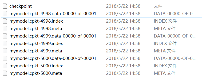
而通常情况下,上述两种通过检查点载入模型参数的结果是一样的,主要是因为不管用户保存了多少个模型文件,都会被记录在唯一一个检查点文件中,这个指定保存模型个数的参数就是max_to_keep,例如:
saver = tf.train.Saver(max_to_keep=3)
而检查点都会默认用最新的模型载入,忽略了之前的模型,因此上述两个检查点载入了同一个模型,自然最后输出的测试结果是一致的。保存的三个模型如图:
接下来,为什么上面的变量,需要给它对应的操作起个名字,而且是不一样的名字呢?像weight1、bias1等等。大家都知道,名字这个东西太重要了,通过它可以访问我们想访问的变量,也就可以对其进行一些操作。例如:
- 显示模型的内容
不同版本的函数会有些区别,本文试验的版本是1.7.0,代码例如:
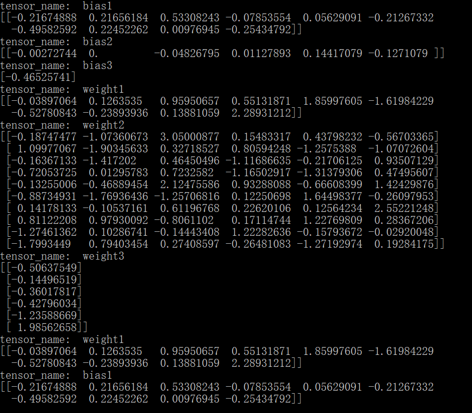
# -*- coding: utf-8 -*-
import tensorflow as tf
from tensorflow.python.tools import inspect_checkpoint as chkp

#显示全部变量的名字和值
chkp.print_tensors_in_checkpoint_file("model/mymodel.cpkt-5000", all_tensor_names='', tensor_name='', all_tensors=True)
#显示指定名字变量的值
chkp.print_tensors_in_checkpoint_file("model/mymodel.cpkt-5000", all_tensor_names='', tensor_name='weight1', all_tensors=False)
chkp.print_tensors_in_checkpoint_file("model/mymodel.cpkt-5000", all_tensor_names='', tensor_name='bias1', all_tensors=False)
运行结果如下图:
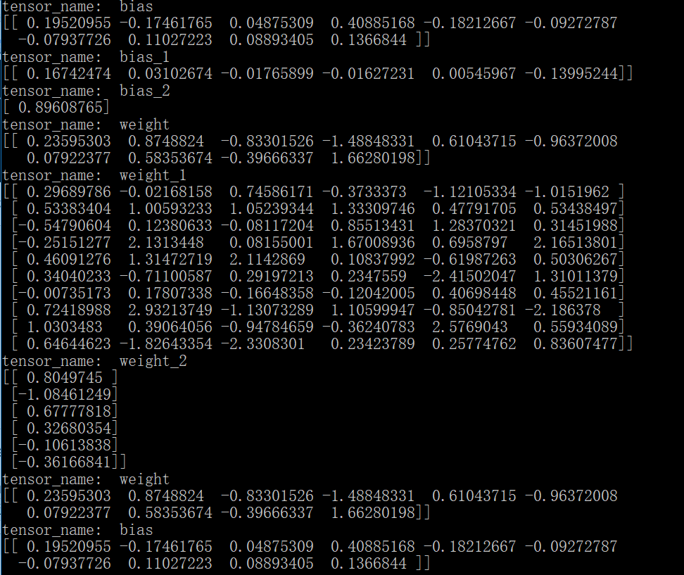
相反如果对不同变量的操作用了同一个name,系统将会自动对同名称操作排序,例如:
# -*- coding: utf-8 -*-
import tensorflow as tf
from tensorflow.python.tools import inspect_checkpoint as chkp

#显示全部变量的名字和值
chkp.print_tensors_in_checkpoint_file("model/mymodel.cpkt-50", all_tensor_names='', tensor_name='', all_tensors=True)
#显示指定名字变量的值
chkp.print_tensors_in_checkpoint_file("model/mymodel.cpkt-50", all_tensor_names='', tensor_name='weight', all_tensors=False)
chkp.print_tensors_in_checkpoint_file("model/mymodel.cpkt-50", all_tensor_names='', tensor_name='bias', all_tensors=False)
结果为:
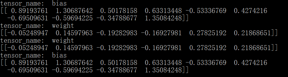
需要注意的是因为对所有同名的变量排序之后,真正的变量名已经变了,所以,当指定查看某一个变量的值时,其实输出的是第一个变量的值,因为它的名称还保留着不变。另外,也可以通过变量的name属性查看其操作名。
- 按名字保存变量
可以通过指定名称来保存变量;注意如果名字如果搞混了,名称所对应的值也就搞混了,比如:
#只保存这两个变量,并且这两个被搞混了
saver = tf.train.Saver({'weight': parameter['b2'], 'bias':parameter['W1']})

# -*- coding: utf-8 -*-
import tensorflow as tf
from tensorflow.python.tools import inspect_checkpoint as chkp

#显示全部变量的名字和值
chkp.print_tensors_in_checkpoint_file("model/mymodel.cpkt-50", all_tensor_names='', tensor_name='', all_tensors=True)
#显示指定名字变量的值
chkp.print_tensors_in_checkpoint_file("model/mymodel.cpkt-50", all_tensor_names='', tensor_name='weight', all_tensors=False)
chkp.print_tensors_in_checkpoint_file("model/mymodel.cpkt-50", all_tensor_names='', tensor_name='bias', all_tensors=False)
此时的结果是:
这样,模型按照我们的想法保存了参数,注意不能搞混变量和其对应的名字。