含并行连接的网络(GoogLeNet)
在2014年的ImageNet图像识别挑战赛中,一个名叫GoogLeNet (Szegedy et al., 2015)的网络架构大放异彩。 GoogLeNet吸收了NiN中串联网络的思想,并在此基础上做了改进。 这篇论文的一个重点是解决了什么样大小的卷积核最合适的问题。 毕竟,以前流行的网络使用小到\(1\times1\),大到\(11\times11\)的卷积核。 本文的一个观点是,有时使用不同大小的卷积核组合是有利的。 下面将介绍一个稍微简化的GoogLeNet版本:我们省略了一些为稳定训练而添加的特殊特性,现在有了更好的训练方法,这些特性不是必要的。
Inception块
在GoogLeNet中,基本的卷积块被称为Inception块(Inception block)。这很可能得名于电影《盗梦空间》(Inception),因为电影中的一句话“我们需要走得更深”(“We need to go deeper”)。
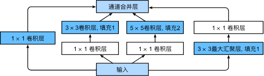
如上图所示,Inception块由四条并行路径组成。 前三条路径使用窗口大小为\(1\times1\)、\(3\times3\)和\(5\times5\)的卷积层,从不同空间大小中提取信息。 中间的两条路径在输入上执行\(1\times1\)卷积,以减少通道数,从而降低模型的复杂性。 第四条路径使用\(3\times3\)最大汇聚层,然后使用\(1\times1\)卷积层来改变通道数。 这四条路径都使用合适的填充来使输入与输出的高和宽一致,最后我们将每条线路的输出在通道维度上连结,并构成Inception块的输出。在Inception块中,通常调整的超参数是每层输出通道数。
import torch
from torch import nn
from torch.nn import functional as F
from d2l import torch as d2l

class Inception(nn.Module):
    def __init__(self, in_channels, c1, c2, c3, c4, **kwargs):
        super(Inception, self).__init__(**kwargs)
        # 1x1 convolution branch
        self.p1_1 = nn.Conv2d(in_channels, c1, kernel_size=1)
        # 1x1 convolution branch followed by 3x3 convolution branch
        self.p2_1 = nn.Conv2d(in_channels, c2[0], kernel_size=1)
        self.p2_2 = nn.Conv2d(c2[0], c2[1], kernel_size=3, padding=1)
        # 1x1 convolution branch followed by 5x5 convolution branch
        self.p3_1 = nn.Conv2d(in_channels, c3[0], kernel_size=1)
        self.p3_2 = nn.Conv2d(c3[0], c3[1], kernel_size=5, padding=2)
        # Max pooling branch followed by 1x1 convolution branch
        self.p4_1 = nn.MaxPool2d(kernel_size=3, stride=1, padding=1)
        self.p4_2 = nn.Conv2d(in_channels, c4, kernel_size=1)

    def forward(self, x):
        # Forward pass through each branch and apply activation function
        p1 = F.relu(self.p1_1(x))
        p2 = F.relu(self.p2_2(F.relu(self.p2_1(x))))
        p3 = F.relu(self.p3_2(F.relu(self.p3_1(x))))
        p4 = F.relu(self.p4_2(self.p4_1(x)))
        # Concatenate the outputs from all branches along the channel dimension
        return torch.cat((p1, p2, p3, p4), dim=1)
那么为什么GoogLeNet这个网络如此有效呢? 首先我们考虑一下滤波器(filter)的组合,它们可以用各种滤波器尺寸探索图像,这意味着不同大小的滤波器可以有效地识别不同范围的图像细节。 同时,我们可以为不同的滤波器分配不同数量的参数。
GoogLeNet模型
如下图所示,GoogLeNet一共使用9个Inception块和全局平均汇聚层的堆叠来生成其估计值。Inception块之间的最大汇聚层可降低维度。 第一个模块类似于AlexNet和LeNet,Inception块的组合从VGG继承,全局平均汇聚层避免了在最后使用全连接层。
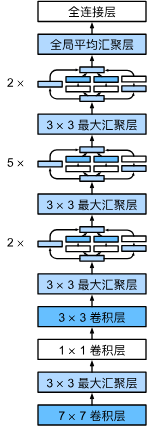
现在,我们逐一实现GoogLeNet的每一个模块。第一个模块使用64个通道,\(7\times7\)卷积层。
# Define a sequential neural network module with a 2D convolutional layer
# input channels=1, output channels=64, kernel size=7, stride=2, padding=3
# followed by a Rectified Linear Unit (ReLU) activation function
# and a 2D max pooling layer with kernel size=3, stride=2, padding=1
b1 = nn.Sequential(nn.Conv2d(1, 64, kernel_size=7, stride=2, padding=3),
                   nn.ReLU(),
                   nn.MaxPool2d(kernel_size=3, stride=2, padding=1))
第二个模块使用两个卷积层:第一个卷积层是64个通道、\(1\times1\)卷积层;第二个卷积层使用将通道数量增加三倍的\(3\times3\)卷积层。 这对应于Inception块中的第二条路径。
# Define a sequential neural network module with the following layers:
b2 = nn.Sequential(
    nn.Conv2d(64, 64, kernel_size=1),  # 1st convolutional layer with 64 input and 64 output channels using a 1x1 kernel
    nn.ReLU(),  # ReLU activation function
    nn.Conv2d(64, 192, kernel_size=3, padding=1),  # 2nd convolutional layer with 64 input and 192 output channels using a 3x3 kernel with padding
    nn.ReLU(),  # ReLU activation function
    nn.MaxPool2d(kernel_size=3, stride=2, padding=1)  # Max pooling layer with a 3x3 kernel, stride of 2, and padding of 1
)
第三个模块串联两个完整的Inception块。 第一个Inception块的输出通道数为\(64+128+32+32=256\),四个路径之间的输出通道数量比为\(64:128:32:32=2:4:1:1\)。 第二个和第三个路径首先将输入通道的数量分别减少到\(96/192=1/2\)和\(16/192=1/12\),然后连接第二个卷积层。第二个Inception块的输出通道数增加到\(128+192+96+64=480\),四个路径之间的输出通道数量比为\(128:192:96:64 = 4:6:3:2\)。 第二条和第三条路径首先将输入通道的数量分别减少到\(128/256=1/2\)和\(32/256=1/8\)。
# Define a nn.Sequential module with three Inception modules and a MaxPool2d layer
b3 = nn.Sequential(Inception(192, 64, (96, 128), (16, 32), 32),
                  Inception(256, 128, (128, 192), (32, 96), 64),
                  nn.MaxPool2d(kernel_size=3, stride=2, padding=1))
第四模块更加复杂, 它串联了5个Inception块,其输出通道数分别是\(192+208+48+64=512\)、\(160+224+64+64=512\)、\(128+256+64+64=512\)、\(112+288+64+64=528\)和\(256+320+128+128=832\)。 这些路径的通道数分配和第三模块中的类似,首先是含\(3×3\)卷积层的第二条路径输出最多通道,其次是仅含\(1×1\)卷积层的第一条路径,之后是含\(5×5\)卷积层的第三条路径和含\(3×3\)最大汇聚层的第四条路径。 其中第二、第三条路径都会先按比例减小通道数。 这些比例在各个Inception块中都略有不同。
# Define a nn.Sequential module with multiple Inception modules and a MaxPool2d layer
b4 = nn.Sequential(Inception(480, 192, (96, 208), (16, 48), 64),
                   Inception(512, 160, (112, 224), (24, 64), 64),
                   Inception(512, 128, (128, 256), (24, 64), 64),
                   Inception(512, 112, (144, 288), (32, 64), 64),
                   Inception(528, 256, (160, 320), (32, 128), 128),
                   nn.MaxPool2d(kernel_size=3, stride=2, padding=1))
第五模块包含输出通道数为\(256+320+128+128=832\)和\(384+384+128+128=1024\)的两个Inception块。 其中每条路径通道数的分配思路和第三、第四模块中的一致,只是在具体数值上有所不同。 需要注意的是,第五模块的后面紧跟输出层,该模块同NiN一样使用全局平均汇聚层,将每个通道的高和宽变成1。 最后我们将输出变成二维数组,再接上一个输出个数为标签类别数的全连接层。
# Define a Sequential module 'b5' consisting of multiple Inception modules and adaptive average pooling
b5 = nn.Sequential(Inception(832, 256, (160, 320), (32, 128), 128),
                  Inception(832, 384, (192, 384), (48, 128), 128),
                  nn.AdaptiveAvgPool2d((1, 1)),
                  nn.Flatten())

# Define the final neural network model 'net' as a Sequential module consisting of previously defined modules and a linear layer
net = nn.Sequential(b1, b2, b3, b4, b5, nn.Linear(1024, 10))
GoogLeNet模型的计算复杂,而且不如VGG那样便于修改通道数。 为了使Fashion-MNIST上的训练短小精悍,我们将输入的高和宽从224降到96,这简化了计算。下面演示各个模块输出的形状变化。
X = torch.rand(size=(1, 1, 96, 96))
for layer in net:
    X = layer(X)
    print(layer.__class__.__name__,'output shape:\t', X.shape)
Sequential output shape:	 torch.Size([1, 64, 24, 24])
Sequential output shape:	 torch.Size([1, 192, 12, 12])
Sequential output shape:	 torch.Size([1, 480, 6, 6])
Sequential output shape:	 torch.Size([1, 832, 3, 3])
Sequential output shape:	 torch.Size([1, 1024])
Linear output shape:	 torch.Size([1, 10])
训练模型
和以前一样,我们使用Fashion-MNIST数据集来训练我们的模型。在训练之前,我们将图片转换为\(96\times96\)分辨率。
lr, num_epochs, batch_size = 0.1, 10, 128
train_iter, test_iter = d2l.load_data_fashion_mnist(batch_size, resize=96)
d2l.train_ch6(net, train_iter, test_iter, num_epochs, lr, d2l.try_gpu())
loss 0.242, train acc 0.908, test acc 0.887
1277.4 examples/sec on cuda:0


 浙公网安备 33010602011771号