
[转]python (matplotlib)画三维图像
[转]python (matplotlib)画三维图像
觉得有用的话,欢迎一起讨论相互学习~


版权声明:本文为CSDN博主「Mr-Cat伍可猫」的原创文章,遵循CC 4.0 BY-SA版权协议,转载请附上原文出处链接及本声明。
原文链接:https://blog.csdn.net/Mr_Cat123/article/details/100054757
文章目录
关于三维图像的内容很多博友已经写了
推荐: 三维绘图, 画三维图, 3d图-英文版, 中文版三维图
上面写的都非常详细,很推荐,特别是英文版和中文版三维图那个,基于此,只给我写的一个例子
1 三维图
画 f ( x , y ) = x 2 + y 2 f(x,y)=x^2+y^2 f(x,y)=x2+y2的三维图

import numpy as np
import matplotlib.pyplot as plt
from mpl_toolkits.mplot3d import Axes3D

x = np.arange(-10,10,0.2)
y = np.arange(-10,10,0.2)
f_x_y=np.power(x,2)+np.power(y,2)
fig = plt.figure()
ax = plt.gca(projection='3d')
ax.plot(x,y,f_x_y)
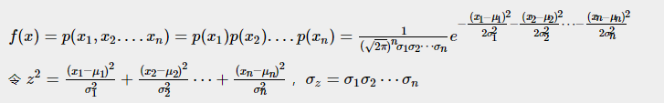
画出2维不相关高斯分布的3维图,即下面公式中n=2的情况

import numpy as np
import matplotlib.pyplot as plt
import mpl_toolkits.axisartist as axisartist
from mpl_toolkits.mplot3d import Axes3D #画三维图不可少
from matplotlib import cm  #cm 是colormap的简写

# 1_dimension gaussian function
def gaussian(x,mu,sigma):
    f_x = 1/(sigma*np.sqrt(2*np.pi))*np.exp(-np.power(x-mu, 2.)/(2*np.power(sigma,2.)))
    return(f_x)

# 2_dimension gaussian function
def gaussian_2(x,y,mu_x,mu_y,sigma_x,sigma_y):
    f_x_y = 1/(sigma_x*sigma_y*(np.sqrt(2*np.pi))**2)*np.exp(-np.power\
              (x-mu_x, 2.)/(2*np.power(sigma_x,2.))-np.power(y-mu_y, 2.)/\
              (2*np.power(sigma_y,2.)))
    return(f_x_y)

#设置2维表格
x_values = np.linspace(-5,5,2000)
y_values = np.linspace(-5,5,2000)
X,Y = np.meshgrid(x_values,y_values)
#高斯函数
mu_x,mu_y,sigma_x,sigma_y = 0,0,0.8,0.8
F_x_y = gaussian_2(X,Y,mu_x,mu_y,sigma_x,sigma_y)
#显示三维图
fig = plt.figure()
ax = plt.gca(projection='3d')
ax.plot_surface(X,Y,F_x_y,cmap='jet')
# 显示等高线图
#ax.contour3D(X,Y,F_x_y,50,cmap='jet')
2 三维等高线
将上面等高线打开,三维图注释掉
#ax.plot_surface(X,Y,F_x_y,cmap='jet')
# 显示等高线图
ax.contour3D(X,Y,F_x_y,50,cmap='jet')

3 二维等高线
将上面的图截取截面就是2维平面,是一个个圆形

import numpy as np
import matplotlib.pyplot as plt
import mpl_toolkits.axisartist as axisartist
from mpl_toolkits.mplot3d import Axes3D #画三维图不可少
from matplotlib import cm  #cm 是colormap的简写

#定义坐标轴函数
def setup_axes(fig, rect):
    ax = axisartist.Subplot(fig, rect)
    fig.add_axes(ax)

    ax.set_ylim(-4, 4)
    #自定义刻度
#    ax.set_yticks([-10, 0,9])
    ax.set_xlim(-4,4)
    ax.axis[:].set_visible(False)

	#第2条线,即y轴,经过x=0的点
    ax.axis["y"] = ax.new_floating_axis(1, 0)
    ax.axis["y"].set_axisline_style("-|>", size=1.5)
#    第一条线,x轴,经过y=0的点
    ax.axis["x"] = ax.new_floating_axis(0, 0)
    ax.axis["x"].set_axisline_style("-|>", size=1.5)

    return(ax)
# 1_dimension gaussian function
def gaussian(x,mu,sigma):
    f_x = 1/(sigma*np.sqrt(2*np.pi))*np.exp(-np.power(x-mu, 2.)/(2*np.power(sigma,2.)))
    return(f_x)

# 2_dimension gaussian function
def gaussian_2(x,y,mu_x,mu_y,sigma_x,sigma_y):
    f_x_y = 1/(sigma_x*sigma_y*(np.sqrt(2*np.pi))**2)*np.exp(-np.power\
              (x-mu_x, 2.)/(2*np.power(sigma_x,2.))-np.power(y-mu_y, 2.)/\
              (2*np.power(sigma_y,2.)))
    return(f_x_y)

#设置画布
fig = plt.figure(figsize=(8, 8)) #建议可以直接plt.figure()不定义大小
ax1 = setup_axes(fig, 111)
ax1.axis["x"].set_axis_direction("bottom")
ax1.axis['y'].set_axis_direction('right')
#在已经定义好的画布上加入高斯函数
x_values = np.linspace(-5,5,2000)
y_values = np.linspace(-5,5,2000)
X,Y = np.meshgrid(x_values,y_values)
mu_x,mu_y,sigma_x,sigma_y = 0,0,0.8,0.8
F_x_y = gaussian_2(X,Y,mu_x,mu_y,sigma_x,sigma_y)
#显示三维图
#fig = plt.figure()
#ax = plt.gca(projection='3d')
#ax.plot_surface(X,Y,F_x_y,cmap='jet')
# 显示3d等高线图
#ax.contour3D(X,Y,F_x_y,50,cmap='jet')
# 显示2d等高线图,画8条线
plt.contour(X,Y,F_x_y,8)
4 三维表面图上画曲线
fig = plt.figure()
ax = fig.gca(projection='3d')
temp_test = np.squeeze(temp[:,0,:,:])
Lat,Lon = np.meshgrid(lat,lon)
# Temp = np.zeros((lat.size,lon.size))
Temp = temp_test[0]    #first hour
surf = ax.plot_surface(Lat,Lon,Temp)
fig.colorbar=(surf)  #画表面图
ax.plot(lat_new, lon_new, t_interp,linewidth=10,color='r')  #画曲线

plt.show()
由于我的值结果范围太小,看不出来,这条曲线是在表面上画一个环


5 三维曲线投影到坐标轴
由于三维曲面投影到坐标轴已经有了答案,在一开始我给的链接或者官网都有,如下:

(代码可以点开始给的链接进入查看)
但是三维 曲 线 曲线 曲线的投影还没有给,所以这里通过查找一番之后总结如下(参考python,matlab)
以下我使用的是python
import matplotlib.pyplot as plt
fig = plt.figure()
ax = fig.gca(projection='3d')
#输入经纬度和海拔值(也就是x,y,z)
ax.plot(lat_new, lon_new, temp_list[layer], linewidth=10, color='r')

plt.show()

现在要将这个图投影到x-z坐标面上
fig = plt.figure()
ax = fig.gca(projection='3d')
ax.plot(lat_new, lon_new, temp_list[layer], linewidth=10, color='r')
null = [30]*len(lat_new)  #在y=30处的面

ax.plot(null, lon_new, temp_list[layer])
# ax.plot(lat_new,null, temp_list[layer])
# ax.plot(lat_new, lon_new, null)

plt.show()

同时在三个面上投影
fig = plt.figure()
ax = fig.gca(projection='3d')
ax.plot(lat_new, lon_new, temp_list[layer], linewidth=10, color='r')
#至于要在多大的值上投影,可以自己测试找到最合适的
x_z = [min(lat_new)-0.5]*len(lat_new)
y_z = [max(lon_new)+0.5]*len(lon_new)
x_y = [min(temp_list[layer])-0.5]*len(temp_list[layer])

ax.plot(x_z, lon_new, temp_list[layer])
ax.plot(lat_new, y_z, temp_list[layer])
ax.plot(lat_new, lon_new, x_y)

plt.show()


 浙公网安备 33010602011771号