动手学深度学习_3 线性神经网络

summer pocket_久岛鸥 我将会跨越七大洋，将我的爱意带到你的身边

---

线性回归基本概念

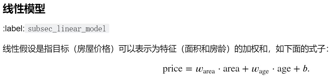
这里的price泛化后就是我们的y，即标签label
这里的area,age泛化后就是我们的X，即特征features

• 当L（W，b）能够通过直接求导得到W与b,那么我们称之W与b有解析解（因为L（W,b）是一个凸函数，当求导后令导数为0,求出的W与b就是使得L（w,b）最小的参数）
  
  
  

• 
  这里公式上的n为学习率，他是代表在梯度方向上走的“步长”
  后面看起来比较复杂的导数其实是在说明
  

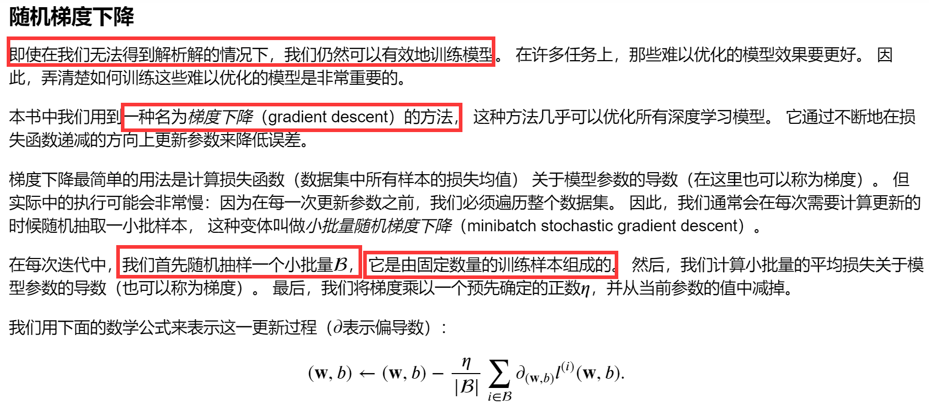
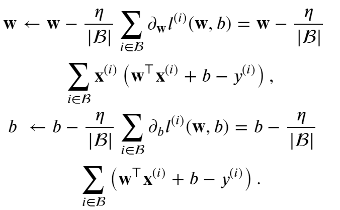
梯度是指函数数值增长最大的方向
当梯度前面有负号，则是说明指向函数数值减少最大的方向
上面的操作都是让参数w与b向着让L（W，b）最大减少的方向变化的

线性回归的从零开始实现

• 生成数据集
• 读取数据集
• 初始化模型参数
• 定义模型
• 定义损失函数
• 定义优化算法
• 训练

上述过程是一般的深度学习的一般过程
因为我们没有数据，需要用正则表达式函数创建数据所以有生成数据集这个步骤

生成数据集

%matplotlib inline
import random
import torch
from d2l import torch as d2l
 
#生成数据，这里模拟出来的是真实的y,x
def synthetic_data(w, b, num_examples):  #@save
    """生成y=Xw+b+噪声"""
    X = torch.normal(0, 1, (num_examples, len(w))) 
    y = torch.matmul(X, w) + b
    y += torch.normal(0, 0.01, y.shape)
    return X, y.reshape((-1, 1))
 
true_w = torch.tensor([2, -3.4])
true_b = 4.2
#一共模拟出1000个点，得到X=features(特征)，Y=labels(标签)
features, labels = synthetic_data(true_w, true_b, 1000)
 
# 画出上述生成的数据
d2l.set_figsize()
d2l.plt.scatter(features[:, 0].detach().numpy(), labels.detach().numpy(), 1);
d2l.plt.scatter(features[:, 1].detach().numpy(), labels.detach().numpy(), 1);
 

这一步中我们先设定出W与b，然后利用随机函数求出X，利用y=WX+b求出y
下面我们可以利用得出的数据X，y进行线性回归，用线性回归得出的W与b,和我们设置的W与b进行比较，差距越小，说明线性回归的效果越好

读取数据集

'''
训练模型时要对数据集进行遍历，每次抽取一小批量样本，并使用它们来更新我们的模型。 
由于这个过程是训练机器学习算法的基础，所以有必要定义一个函数， 该函数能打乱数据集中的样本并以小批量方式获取数据。
'''
# 读取数据
# 这个函数的作用就真是每一次从features和labels中随机取出batch_size个数据点出来
def data_iter(batch_size,features,labels):
    num_examples=len(features)
    print(f'len(features):{len(features)}\n')
    indices=list(range(num_examples))
    random.shuffle(indices)
    for i in range(0,num_examples,batch_size):
        batch_indices=torch.tensor(
            indices[i:min(i+batch_size,num_examples)])
        yield features[batch_indices],labels[batch_indices]
 
batch_size = 10        
 

• range函数：range(start, stop[, step])
• 令人震惊的是 features[batch_indices] , labels[batch_indices] 的用法，居然可以使用张量batch_indices作为下标一次取多个值
• num_examples=len(features): features是个矩阵，len(features)得出的是其行数
• batch_indices=torch.tensor(indices[i:min(i+batch_size,num_examples)]) 其中i:min(i+batch_size,num_examples)利用的是切片技术

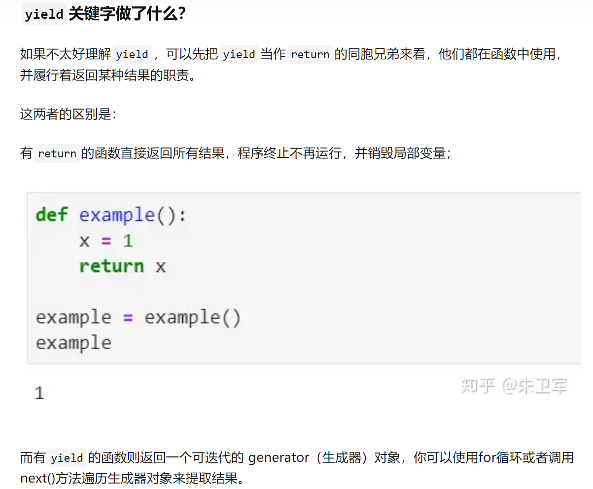
• yield：
  就是可以简单地理解为yield是用来返回的，但是返回后函数中的状态不会销毁，下次使用next()或for再次执行时，可以接着原来的状态继续执行

如：

for X, y in data_iter(batch_size, features, labels):
    print(X, '\n', y)
    break

上述就是调用函数的一种方式

---

• 如果是用框架代码实现的话

from torch.utils import data
def load_array(data_arrays, batch_size, is_train=True):  #@save
    """构造一个PyTorch数据迭代器"""
    dataset = data.TensorDataset(*data_arrays)
    return data.DataLoader(dataset, batch_size, shuffle=is_train)
data_iter = load_array((features, labels), batch_size)

data_arrays是一个元组，元组中的元素是张量，通过 data.TensorDataset（）生成dataset,并结合data.DataLoader返回一个数据生成器，与yeild有着相同的效果。

初始化模型参数

# 初始化模型参数
w=torch.normal(0,0.01,size=(2,1),requires_grad=True)
b=torch.zeros(1,requires_grad=True)

• 如果是用框架写：
  net是下面用框架定义的nn.Sequential(nn.Linear(2, 1))

net[0].weight.data.normal_(0, 0.01)
net[0].bias.data.fill_(0)

定义模型

#定义模型
def linreg(X,w,b): #@save
    return torch.matmul(X,w)+b

• 如果是用框架写：

# nn是神经网络的缩写
from torch import nn
 
net = nn.Sequential(nn.Linear(2, 1))

定义损失函数

# 定义损失函数
def squared_loss(y_hat,y):#@save
    return (y_hat-y.reshape(y_hat.shape))**2/2

• 如果是用框架写：

loss = nn.MSELoss()

定义优化算法

# 定义优化算法
#batch_size为样本个数
def sgd(params,lr,batch_size):#@save
    with torch.no_grad():
        for param in params:
            param -= lr*param.grad/batch_size
            param.grad.zero_()

• 框架代码写：

trainer = torch.optim.SGD(net.parameters(), lr=0.03)

训练

# 训练
 
# 先定义参数
lr=0.03 #学习率
num_epochs=3 #训练次数
net=linreg
loss=squared_loss
 
for epoch in range(num_epochs):
    for X,y in data_iter(batch_size,features,labels):
        l=loss(net(X,w,b),y)
        l.sum().backward()
        sgd([w,b],lr,batch_size)
    with torch.no_grad():
        train_l=loss(net(features,w,b),labels)
        print(f'epoch {epoch+1},loss {float(train_l.mean()):f}')
 

softmax 回归

其首先是一个分类问题：

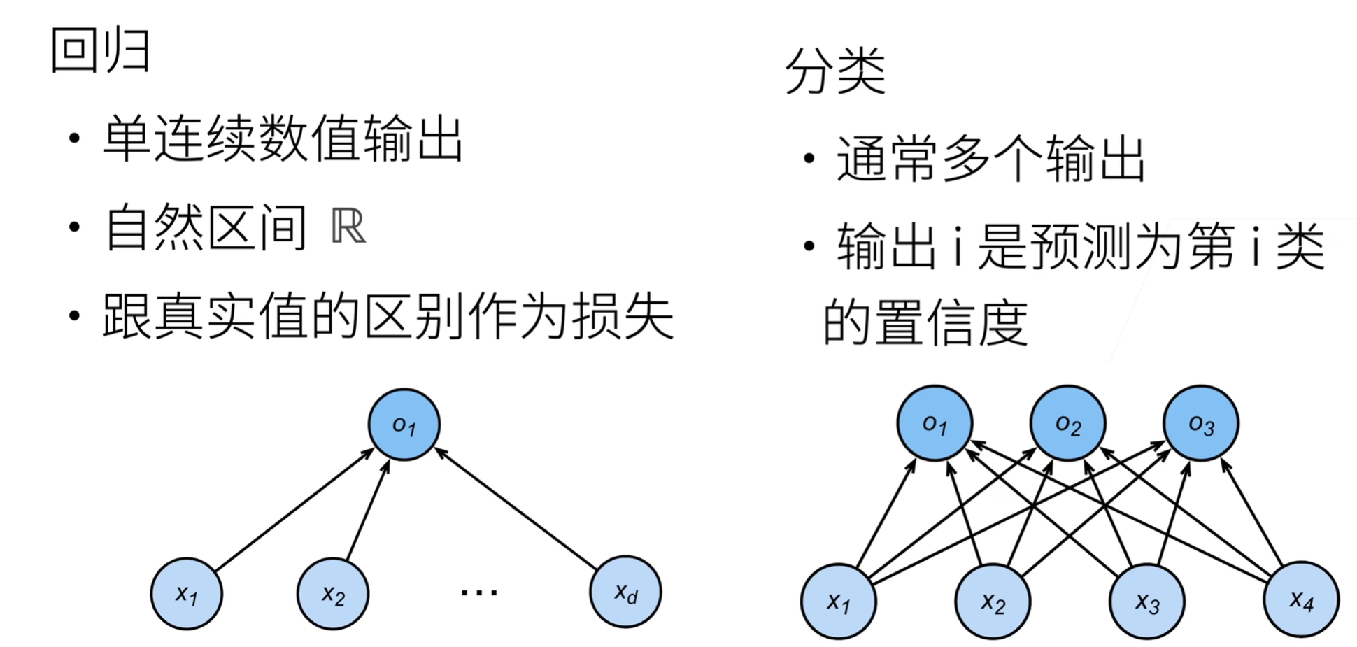
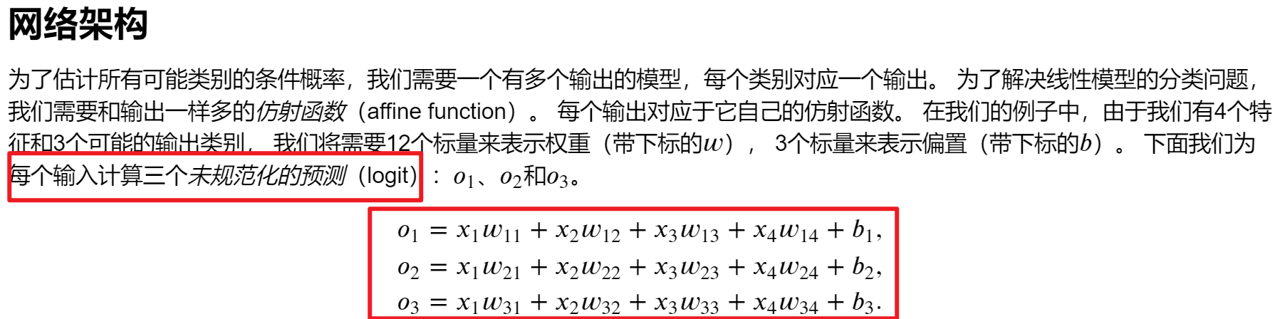
• 模型
  

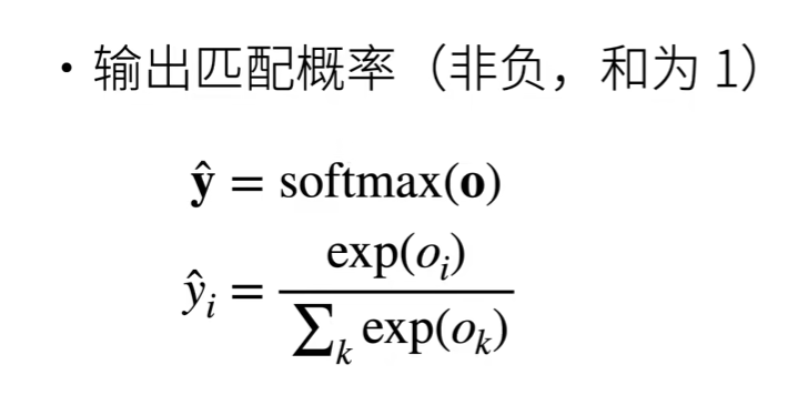
softmax操作其实就是相当于一种归一化操作

• 损失函数
  
  

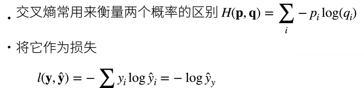
这个概率y是指对于某一个物品我们要模型将他分为4类(假设)
对于这个物品我们其实一开始就知道了他是某一类，假设这里他是第1类
那么y为[1,0,0,0]
对于y_hat，他是模型求出来的可能是y_hat=[0.5,0.3,0.2,0.1]
我们用交叉熵公式去求，发现其实y只有1个为1，其余为0
那么交叉熵公式就可以化简为-logy_haty(即表示对应着y为1的那个下标)

代码实现

import torch
from IPython import display
from d2l import torch as d2l
# 读取数据
'''
现在我们[定义load_data_fashion_mnist函数]，用于获取和读取Fashion-MNIST数据集。 
这个函数返回训练集和验证集的数据迭代器。 
此外，这个函数还接受一个可选参数resize，用来将图像大小调整为另一种形状。
'''
def load_data_fashion_mnist(batch_size, resize=None):  #@save
    """下载Fashion-MNIST数据集，然后将其加载到内存中"""
    trans = [transforms.ToTensor()]
    if resize:
        trans.insert(0, transforms.Resize(resize))
    trans = transforms.Compose(trans)
    mnist_train = torchvision.datasets.FashionMNIST(
        root="../data", train=True, transform=trans, download=True)
    mnist_test = torchvision.datasets.FashionMNIST(
        root="../data", train=False, transform=trans, download=True)
    return (data.DataLoader(mnist_train, batch_size, shuffle=True,
                            num_workers=get_dataloader_workers()),
            data.DataLoader(mnist_test, batch_size, shuffle=False,
                            num_workers=get_dataloader_workers()))
 
batch_size = 256
# 如果对load_data_fashion_mnist不添加resize参数，那么就是默认28x28的图片，同时通道数为1
train_iter, test_iter = d2l.load_data_fashion_mnist(batch_size)
 
 
# 初始化模型参数
num_inputs=784 #784即是28*28,这个要联合software回归的线性回归方程才能理解
num_outputs=10
 
W=torch.normal(0,0.01,size=(num_inputs,num_outputs),requires_grad=True)# W为torch.Size([784, 10])
b=torch.zeros(num_outputs,requires_grad=True)# b为torch.Size([10])
 
# 定义模型
def software(X): # 首先定义下对于数值归一化的software操作
    # 那么根据下面的分析，这里就是要对256x10的矩阵中的每一行进行software操作，使得每一行数据相加为1
    X_exp=torch.exp(X)
    partition=X_exp.sum(1,keepdim=True)
    return X_exp/partition # partition 是X每一行的和，利用广播机制可以让每一行除上对应的总和
    
def net(X):
    #The expression W.shape[0] typically refers to the number of rows in a matrix 
    #X.reshape((-1,W.shape[0])).shape:torch.Size([256, 784])
    #这里得出来的矩阵为256x10,即行意味着每一张图片，共有256张图片，列表示模型对这张图片分成不同类的概率
    return software(torch.matmul(X.reshape((-1,W.shape[0])),W)+b)
 
# 定义损失函数
def cross_entropy(y_hat, y):
    # len(y_hat)为256，y是一个256的向量，其中是表示真正每一张图片真正的类的下标
    #这个函数返回的是一个256的向量，即每一张照片的损失
    return - torch.log(y_hat[range(len(y_hat)), y])
 
# 定义优化函数
lr = 0.1
 
def updater(batch_size):
    return d2l.sgd([W, b], lr, batch_size) # W.grad torch.Size([784, 10]),W本身就是784x10的矩阵，
 
 
# 可视化
class Accumulator:  #@save
    """在n个变量上累加"""
    def __init__(self, n):
        self.data = [0.0] * n
 
    def add(self, *args):
        self.data = [a + float(b) for a, b in zip(self.data, args)]
 
    def reset(self):
        self.data = [0.0] * len(self.data)
 
    def __getitem__(self, idx):
        return self.data[idx]
    
def accuracy(y_hat, y):  #@save
    """计算预测正确的数量"""
    if len(y_hat.shape) > 1 and y_hat.shape[1] > 1:
        y_hat = y_hat.argmax(axis=1)
    cmp = y_hat.type(y.dtype) == y
    return float(cmp.type(y.dtype).sum())
 
def evaluate_accuracy(net, data_iter):  #@save
    """计算在指定数据集上模型的精度"""
    if isinstance(net, torch.nn.Module):
        net.eval()  # 将模型设置为评估模式
    metric = Accumulator(2)  # 正确预测数、预测总数
    with torch.no_grad():
        for X, y in data_iter:
            metric.add(accuracy(net(X), y), y.numel())
    return metric[0] / metric[1]
 
 
class Animator:  #@save
    """在动画中绘制数据"""
    def __init__(self, xlabel=None, ylabel=None, legend=None, xlim=None,
                 ylim=None, xscale='linear', yscale='linear',
                 fmts=('-', 'm--', 'g-.', 'r:'), nrows=1, ncols=1,
                 figsize=(3.5, 2.5)):
        # 增量地绘制多条线
        if legend is None:
            legend = []
        d2l.use_svg_display()
        self.fig, self.axes = d2l.plt.subplots(nrows, ncols, figsize=figsize)
        if nrows * ncols == 1:
            self.axes = [self.axes, ]
        # 使用lambda函数捕获参数
        self.config_axes = lambda: d2l.set_axes(
            self.axes[0], xlabel, ylabel, xlim, ylim, xscale, yscale, legend)
        self.X, self.Y, self.fmts = None, None, fmts
 
    def add(self, x, y):
        # 向图表中添加多个数据点
        if not hasattr(y, "__len__"):
            y = [y]
        n = len(y)
        if not hasattr(x, "__len__"):
            x = [x] * n
        if not self.X:
            self.X = [[] for _ in range(n)]
        if not self.Y:
            self.Y = [[] for _ in range(n)]
        for i, (a, b) in enumerate(zip(x, y)):
            if a is not None and b is not None:
                self.X[i].append(a)
                self.Y[i].append(b)
        self.axes[0].cla()
        for x, y, fmt in zip(self.X, self.Y, self.fmts):
            self.axes[0].plot(x, y, fmt)
        self.config_axes()
        display.display(self.fig)
        display.clear_output(wait=True)
 
# 训练
def train_epoch_ch3(net, train_iter, loss, updater):  #@save
    """训练模型一个迭代周期（定义见第3章）"""
    # 将模型设置为训练模式
    if isinstance(net, torch.nn.Module):
        net.train()
    # 训练损失总和、训练准确度总和、样本数
    metric = Accumulator(3)
    for X, y in train_iter:
        # 计算梯度并更新参数
        y_hat = net(X) # X.shape:torch.Size([256, 1, 28, 28])，y_hat得到的是一个256x10的矩阵
        l = loss(y_hat, y) #y.shape:torch.Size([256]),l.shape:torch.Size([256])
        if isinstance(updater, torch.optim.Optimizer):
            # 使用PyTorch内置的优化器和损失函数
            updater.zero_grad()
            l.mean().backward()
            updater.step()
        else:
            # 使用定制的优化器和损失函数
            l.sum().backward()
            updater(X.shape[0])
        metric.add(float(l.sum()), accuracy(y_hat, y), y.numel())
    # 返回训练损失和训练精度
    return metric[0] / metric[2], metric[1] / metric[2]
 
def train_ch3(net, train_iter, test_iter, loss, num_epochs, updater):  #@save
    """训练模型（定义见第3章）"""
    animator = Animator(xlabel='epoch', xlim=[1, num_epochs], ylim=[0.3, 0.9],
                        legend=['train loss', 'train acc', 'test acc'])
    for epoch in range(num_epochs):
        train_metrics = train_epoch_ch3(net, train_iter, loss, updater)
        test_acc = evaluate_accuracy(net, test_iter)
        animator.add(epoch + 1, train_metrics + (test_acc,))
    train_loss, train_acc = train_metrics
    assert train_loss < 0.5, train_loss
    assert train_acc <= 1 and train_acc > 0.7, train_acc
    assert test_acc <= 1 and test_acc > 0.7, test_acc
 
num_epochs = 10
train_ch3(net, train_iter, test_iter, cross_entropy, num_epochs, updater)

• 框架代码：

import torch
from torch import nn
from d2l import torch as d2l
 
# 获取数据
batch_size = 256
train_iter, test_iter = d2l.load_data_fashion_mnist(batch_size)
 
# 初始化参数与定义模型
 
net = nn.Sequential(nn.Flatten(), nn.Linear(784, 10))# PyTorch不会隐式地调整输入的形状。因此，
def init_weights(m):# 我们在线性层前定义了展平层（flatten），来调整网络输入的形状
    if type(m) == nn.Linear:
        nn.init.normal_(m.weight, std=0.01)
 
net.apply(init_weights);
 
# 定义损失函数
loss = nn.CrossEntropyLoss(reduction='none')
 
# 定义优化算法
 
trainer = torch.optim.SGD(net.parameters(), lr=0.1)
 
# 训练
num_epochs = 10
d2l.train_ch3(net, train_iter, test_iter, loss, num_epochs, trainer)