使用radarsimpy仿真TDM_MIMO_FCMW雷达

radarsimpy 是一个用于雷达仿真的 Python 库项目。功能齐全，文档完善，很好用。

本文将使用 radarsimpy 对TDM MIMO FCMW 雷达进行仿真，并实践 Range-Doppler 和 Angle-FFT。

创建雷达系统#

创建一个 2T4R 的雷达系统。

• 中心频率 $f_c$ 为 60.5e
• 单 chirp 时长 $Tc$ 为 16e-6
• 整个 chirp 周期时长为 40e-6
• 频率调制范围在 [61e9, 60e9]
• 一帧数量为 512
• 采样率 $f_s$ 为 20e6

关于雷达系统的位置和脉冲信息，可以看后文的图示。

import numpy as np
from radarsimpy import Radar, Transmitter, Receiver
from scipy.constants import speed_of_light

wavelength = speed_of_light / 60.5e9

N_tx = 2
N_rx = 4

tx = []
tx.append(
    dict(
        location=(0, -N_rx / 2 * wavelength, 0),
        delay=0,
    )
)
tx.append(
    dict(
        location=(0, 0, 0),
        delay=20e-6,
    )
)

rx = [dict(location=(0, wavelength / 2 * idx, 0)) for idx in range(N_rx)]


tx = Transmitter(f=[61e9, 60e9], t=16e-6, tx_power=15, prp=40e-6, pulses=512, channels=tx)
rx = Receiver(fs=20e6, noise_figure=8, rf_gain=20, load_resistor=500, baseband_gain=30, channels=rx)

radar = Radar(transmitter=tx, receiver=rx)

显示阵列的位置信息。

import plotly.graph_objs as go
from IPython.display import Image

fig = go.Figure()
fig.add_trace(
    go.Scatter(
        x=radar.radar_prop["transmitter"].txchannel_prop["locations"][:, 1] / wavelength,
        y=radar.radar_prop["transmitter"].txchannel_prop["locations"][:, 2] / wavelength,
        mode='markers',
        name='Transmitter',
        opacity=0.7,
        marker=dict(size=10),
    )
)

fig.add_trace(
    go.Scatter(
        x=radar.radar_prop["receiver"].rxchannel_prop["locations"][:, 1] / wavelength,
        y=radar.radar_prop["receiver"].rxchannel_prop["locations"][:, 2] / wavelength,
        mode='markers',
        opacity=1,
        name='Receiver',
    )
)

fig.update_layout(
    title='Array configuration',
    height=400,
    width=700,
    xaxis=dict(title='y (λ)'),
    yaxis=dict(title='z (λ)', scaleanchor="x", scaleratio=1),
)

fig.show()

创建目标，获得回波数据#

创建一个目标，位于 30m 处、10° 的位置，其相对雷达的速度为 25m/s。

true_theta = [10]
speed = [25]
ranges = [30]
targets = []

for theta, v, r in zip(true_theta, speed, ranges):
    target = dict(
        location=(r * np.cos(np.radians(theta)), r * np.sin(np.radians(theta)), 0),
        speed=(v * np.cos(np.radians(theta)), v * np.sin(np.radians(theta)), 0),
        rcs=10,
        phase=0,
    )
    targets.append(target)

计算回波数据。

from radarsimpy.simulator import simc

data = simc(radar, targets, noise=False)
timestamp = data['timestamp']
baseband = data['baseband']

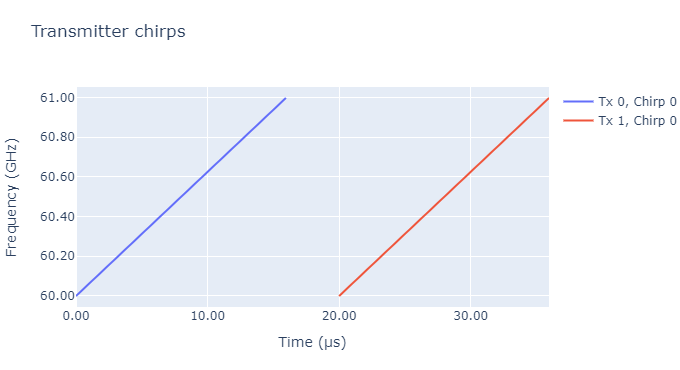
现在让我们看下两个 Tx 天线发射的信号：

# reshaped_timestamp 维度：Tx，Rx，脉冲，采样点
reshaped_timestamp = timestamp.reshape((N_tx, N_rx, 512, -1))

fig = go.Figure()

bandwidth = radar.radar_prop["transmitter"].waveform_prop["bandwidth"]
center_freq = 60.5e9
start_freq = center_freq - bandwidth / 2
stop_freq = center_freq + bandwidth / 2

samples_per_pulse = radar.sample_prop["samples_per_pulse"]

for Tx in range(2):
    x_data = reshaped_timestamp[Tx, 0, 0, :] * 1e6  # x 轴。单位为微秒
    y_data = np.linspace(start_freq, stop_freq, samples_per_pulse, endpoint=False) / 1e9
    trace_name = f'Tx {Tx}, Chirp 0'
    fig.add_trace(go.Scatter(x=x_data, y=y_data, name=trace_name))

fig.update_layout(
    title='Transmitter chirps',
    height=400,
    width=700,
    yaxis=dict(tickformat='.2f', title='Frequency (GHz)'),
    xaxis=dict(tickformat='.2f', title='Time (µs)'),
)

fig.show()

进行 Range-Doppler#

首先定义函数：

def range_fft(X, n=None, window=None):
    if window is not None:
        shape = [1] * X.ndim
        shape[-1] = X.shape[-1]
        X = X * window.reshape(shape)
    output = np.fft.fft(X, n, axis=-1)
    return output


def doppler_fft(X, n=None, window=None):
    if window is not None:
        shape = [1] * X.ndim
        shape[-2] = X.shape[-2]
        X = X * window.reshape(shape)
    output = np.fft.fftshift(np.fft.fft(X, n, axis=-2), axes=-2)
    return output

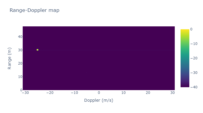
然后进行 Range-Doppler 处理：

from scipy import signal

range_window = signal.windows.chebwin(radar.sample_prop["samples_per_pulse"], at=80)
dop_window = signal.windows.chebwin(radar.radar_prop["transmitter"].waveform_prop["pulses"], at=60)

ranged = range_fft(baseband.conj(), window=range_window)
range_doppler = doppler_fft(ranged, window=dop_window)

绘制处理结果：

from scipy.constants import speed_of_light

max_range = (  # 计算最大探测距离
    speed_of_light  # 光速
    * radar.radar_prop["receiver"].bb_prop["fs"]  # 采样率
    * radar.radar_prop["transmitter"].waveform_prop["pulse_length"]  # 脉冲时长 Tc
    / radar.radar_prop["transmitter"].waveform_prop["bandwidth"]
    / 2
)
range_axis = np.linspace(0, max_range, radar.sample_prop["samples_per_pulse"], endpoint=False)

doppler_axis = np.linspace(
        -1 / radar.radar_prop["transmitter"].waveform_prop["prp"][0] / 2,
        1 / radar.radar_prop["transmitter"].waveform_prop["prp"][0] / 2,
        radar.radar_prop["transmitter"].waveform_prop["pulses"],
        endpoint=False,
    )* speed_of_light / 60.5e9 / 2


fig = go.Figure()
fig.add_trace(
    go.Heatmap(
        z=20 * np.log10(np.mean(np.abs(range_doppler), axis=0)).T,
        x=doppler_axis,
        y=range_axis,
        colorscale='Viridis',
        zmin=-40,
        zmax=0,
    )
)
fig.update_layout(title='Range-Doppler map', xaxis=dict(title='Doppler (m/s)'), yaxis=dict(title='Range (m)'))

fig.show()

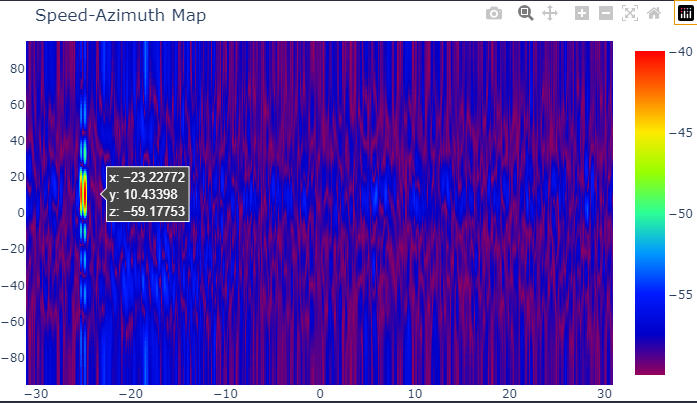
Angle-FFT#

在进行 Angle-FFT 之前，先进行多普勒补偿。

# 获取 dop_bin 长度
dop_bin = np.arange(range_doppler.shape[-2])
# 计算相位差
delta_phi = np.exp(-1j * np.pi * (dop_bin - len(dop_bin) / 2) / len(dop_bin))
# 进行补偿
range_doppler[8:, :, :] *= delta_phi[None, :, None]

然后进行 Angle-FFT 处理：

def angle_fft(X, n=None, window=None):
    if window is not None:
        shape = [1] * X.ndim
        shape[0] = X.shape[0]
        X = X * window.reshape(shape)
    output = np.fft.fftshift(np.fft.fft(X, n, axis=0), axes=0)
    return output

angled = angle_fft(range_doppler, n=128)

绘制一个 Speed-Azimuth 图看效果。下图主要看 y 轴对不对，x 轴我标歪了。

azimuth = np.linspace(-1, 1, 128)
azimuth = np.arcsin(azimuth) / np.pi * 180

fig = go.Figure()
z = 20 * np.log10(np.abs(angled[:, :, 0]) + 0.001)
fig.add_trace(go.Heatmap(x=doppler_axis, y=azimuth, z=z, colorscale='Rainbow'))

fig.update_layout(
    title='Speed-Azimuth Map',
    height=400,
    width=700,
    scene=dict(
        xaxis=dict(title='Doppler (m/s)'),
        yaxis=dict(title='Azimuth (deg)'),
        zaxis=dict(title='Amplitude (dB)'),
        aspectmode='data',
    ),
    margin=dict(l=0, r=0, b=0, t=40),
)

fig.show()

参考来源#

• https://radarsimx.com/2019/04/07/tdm-mimo-fmcw-radar/