Perceptron, Support Vector Machine and Dual Optimization Problem (2)

Generalizing Linear Classification

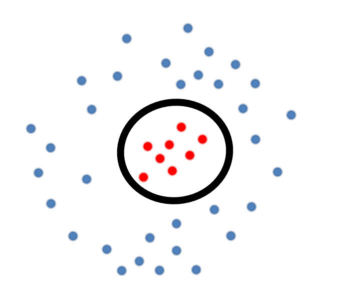
假设我们有如上图的 training data，注意到此时 \(\mathcal{X} \subset \mathbb{R}^{2}\)。

那么 decision boundary \(g\)：

\[g(\vec{x}) = w_{1} x_{1}^{2} + w_{2} x_{2}^{2} + w_{0} \]

即，decision boundary 为某种椭圆，例如：半径为 \(r\) 的圆（\(w_{1} = 1, w_{2} = 1, w_{0}=-r^{2}\)），如上图中的黑圈所示。我们会发现，此时 decision boundary not linear in \(\vec{x}\)。

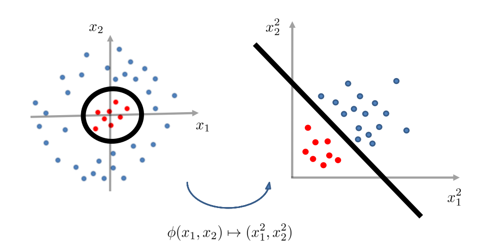
但是，\(g(\vec{x}) = w_{1} x_{1}^{2} + w_{2} x_{2}^{2} + w_{0}\) 在某些空间里却是线性的：

\[\begin{align*} g(\vec{x}) & = w_{1}x_{1}^{2} + w_{2}x_{2}^{2} + w_{0} \qquad \qquad (\text{non-linear in $x_{1}$ and $x_{2}$}) \\ & = w_{1}z_{1} + w_{2}z_{2} + w_{0} \qquad \qquad \; (\text{linear in $z_{1}$ and $z_{2}$}) \end{align*} \]

因此，如果我们对数据进行特征变换（feature transformation）：

\[\phi(x_{1}, x_{2}) \longrightarrow (x_{1}^{2}, x_{2}^{2}) \]

那么 \(g\) 在 \(\phi -\) transformed feature space 中变为线性的。

---

Geometric view on feature transformation

---

Feature Transformation for Quadratic Boundaries

\(\mathbb{R}^{2}-\) case

generic quadratic boundary 如下：

\[\begin{align*} g(\vec{x}) & = w_{1} x_{1}^{2} + w_{2} x_{2}^{2} + w_{3} x_{1} x_{2} + w_{4} x_{1} + w_{5} x_{2} + w_{0} \\ & = \sum\limits_{p + q \leq 2} w^{p, q} x_{1}^{p} x_{2}^{q} \end{align*} \]

feature transformation 则为：

\[\phi(x_{1}, x_{2}) \longrightarrow (x_{1}^{2}, x_{2}^{2}, x_{1}x_{2}, x_{1}, x_{2}, 1) \]

---

\(\mathbb{R}^{d}-\) case

generic quadratic boundary 如下：

\[g(\vec{x}) = \sum\limits_{i, j = 1}^{d} \sum\limits_{p + q \leq 2} w_{i, j}^{p, q}x_{i}^{p}x_{j}^{q} \]

feature transformation 则为：

\[\phi(x_{1}, \ldots, x_{d}) \longrightarrow (x_{1}^{2}, x_{2}^{2}, \ldots, x_{d}^{2}, x_{1}x_{2}, \ldots, x_{d-1} x_{d}, x_{1}, x_{2}, \ldots, x_{d}, 1) \]

• 注意，以上的 \(\mathbb{R}^{2}\) 以及下面会提到的 \(\mathbb{R}^{d}\) 指的是数据的维度。

---

Theorem.

给定 \(n\) 个互不相同的数据点：\(\mathcal{X} = \left\{ \vec{x_{1}}, \vec{x_{2}}, \ldots, \vec{x_{n}} \right\}\)，总是存在一个 feature transformation \(\phi\)，使得无论的 \(\mathcal{S} = \mathcal{X} \times \mathcal{Y}\) 的 label 如何，它在 transformed space 中总是线性可分的。

---

Proof.

给定 \(n\) 个数据点，考虑以下映射（映射至 \(\mathbb{R}^{n}\)）：

\[\phi(\vec{x_{i}}) \longrightarrow \begin{pmatrix} 0 \\ \vdots \\ 0 \\ 1 \\ 0 \\ \vdots \\ 0 \end{pmatrix} \]

即，映射为一个 one-hot 向量，除第 \(i\) 行处为 \(1\)，其它坐标处的值都为 \(0\)。

那么，由 linear weighting \(\vec{w}^{*} = \begin{pmatrix} y_{1} \\ \vdots \\ y_{n} \end{pmatrix}\) 引出的 decision boundary 完美地分割了 input data。

• 解释：

  证明的意思是，输入的数据有 \(n\) 个。对于每一个数据点，feature transform 到一个 one-hot vector，只有这条数据在输入的 \(n\) 个数据中排的位置所对应的坐标处取 \(1\)，其余全部取 \(0\)。假设输入三个数据：\(\vec{x_{1}}, \vec{x_{2}}, \vec{x_{3}}\)，则：

  
  
  \[\phi(\vec{x_{1}}) = \begin{pmatrix} 1 \\ 0 \\ 0 \end{pmatrix} \qquad \phi(\vec{x_{2}}) = \begin{pmatrix} 0 \\ 1 \\ 0 \end{pmatrix} \qquad \phi(\vec{x_{3}}) = \begin{pmatrix} 0 \\ 0 \\ 1 \end{pmatrix} \]

---

这样极端的操作有利有弊：

• 优点：

  
  

  任意的问题都将变为 linear separable。

  
  

• 缺点：

  
  

  1. 计算复杂度：

     
     

     generic kernel transform 的时间复杂度通常是 \(\Omega(n)\)，有些常用的 kernel transform 将 input space 映射到 infinite dimensional space 中。

     
     

  2. 模型复杂度：

     
     

     模型的概括能力（generalization performance）通常随模型复杂度的下降而下降。即，若向简化模型，通常需要以牺牲模型的表现作为代价。

---

• 回顾时间复杂度 \(T(n) = \Omega \big( f(n) \big)\) 的定义：

  
  
  \[\exists c > 0: ~ \exists n_{0} \in \mathbb{N}^{+}: ~ \forall n \geq n_{0}: ~ T(n) \geq c \cdot f(n) \]
  
  

  那么 \(\Omega(n)\) 满足：

  
  
  \[\exists c > 0: ~ \exists n_{0} \in \mathbb{N}^{+}: ~ \forall n \geq n_{0}: ~ T(n) \geq cn \]
  
  

  也就是说时间复杂度最低也与 \(n\) 呈线性。

---

The Kernel Trick (to Deal with Computation)

如果直接暴露在 generic kernel space \(\phi(\vec{x_{i}})\) 中进行运算，需要时间复杂度 \(\Omega(n)\)。但是相对而言地，kernel space 中的两个数据点的点积可以被更快地求出，即：

\[\phi(\vec{x_{i}}) \cdot \phi(\vec{x_{j}}) \]

---

Examples.

• 在 \(\mathbb{R}^{d}\) 空间中的数据的 quadratic kernel transform：

  
  

  • Explicit transform：\(O(d^{2})\)
    
    

    \[\vec{x} \longrightarrow (x_{1}^{2}, \ldots, x_{d}^{2}, \sqrt{2} x_{1} x_{2}, \ldots, \sqrt{2} x_{d-1} x_{d}, \sqrt{2} x_{1}, \ldots, \sqrt{2} x_{d}, 1) \]
    
    

  • Dot products：\(O(d)\)

    
    
    \[(1 + \vec{x_{i}} \cdot \vec{x_{j}})^{2} \]

• 径向基函数（Radial Basis Function, i.e., RBF）：

  
  

  • Explicit transform：infinite dimension！
    
    

    \[\vec{x} \longrightarrow \Big( \big( \frac{2}{\pi} \big)^{\frac{d}{4}} e^{-||\vec{x} - \alpha||^{2}} \Big)_{\alpha \in \mathbb{R}^{d}} \]
    
    

  • Dot products：\(O(d)\)

    \[e^{-||\vec{x_{i}} - \vec{x_{j}}||^{2}} \]

---

Kernel 变换的诀窍在于，在实现分类算法的时候只通过 “点积” 的方式接触数据。

---

Examples.

The Kernel Perceptron（核感知机）

回忆感知机算法，更新权重向量的核心步骤为：

\[\vec{w}^{(t)} \leftarrow \vec{w}^{(t-1)} + y \vec{x} \]

等价地，算法可以写为：

\[\vec{w} = \sum\limits_{k=1}^{n} \alpha_{k} y_{k} \vec{x_{k}} \]

其中，\(\alpha_{k}\) 为在 \(\vec{x_{k}}\) 上发生错误的次数。

因此，分类问题变为：

\[\begin{align*} f(\vec{x}) & = \text{sign}(\vec{w} \cdot \vec{x}) \\ & = \text{sign} \big( \vec{x} \cdot \sum\limits_{k=1}^{n} \alpha_{k} y_{k} \vec{x_{k}} \big) \\ & = \text{sign} \big( \sum\limits_{k=1}^{n} \alpha_{j} y_{k} (\vec{x_{k}} \cdot \vec{x}) \big) \end{align*} \]

其中 \(\vec{x}\) 输入函数 \(f\) 的新数据向量，注意与 \(\vec{x_{k}}\) 区分。

因此，在空间内的分类问题：

\[f(\vec{x}) = \text{sign} \big( \sum\limits_{k=1}^{n} \alpha_{j} y_{k} (\vec{x_{k}} \cdot \vec{x}) \big) \]

若在 tranformed kernel space 中处理，则：

\[f\big( \phi(\vec{x}) \big) = \text{sign} \Big( \sum\limits_{k=1}^{n} \alpha_{k} y_{k} \big( \phi(\vec{x_{k}}) \cdot \phi(\vec{x}) \big) \Big) \]

算法具体如下：

\[\begin{align*} & \text{Initialize}: \vec{\alpha} = \vec{0} \\ & \\ & \text{for } t = 1, 2, 3, \cdots, T: \\ & \\ & \qquad \text{若存在} (\vec{x_{i}}, y) \in \mathcal{S} \text{ s.t. : } \text{sign} \Big( \sum\limits_{k=1}^{n} \alpha_{k} y_{k} \big( \phi(\vec{x_{k}}) \cdot \phi(\vec{x_{i}}) \big) \Big) \neq y_{i}: \\ & \qquad \qquad \alpha_{i} \leftarrow \alpha_{i} + 1 \end{align*} \]

在最后注意到，\(\sum\limits_{k=1}^{n} \alpha_{k} y_{k} \big( \phi(\vec{x_{k}}) \cdot \phi(\vec{x}) \big)\) 中的点积 \(\phi(\vec{x_{k}}) \cdot \phi(\vec{x})\) 是相似度（similarity）的一种衡量方式，故自然能够被其它自定义的相似度衡量方式所替换。

所以，我们可以在任意自定义的非线性空间中，隐性地（implicitly）进行运算，而不需要承担可能的巨大计算量成本。