
KNN算法的实现(R语言)
一 . K-近邻算法(KNN)概述
最简单最初级的分类器是将全部的训练数据所对应的类别都记录下来,当测试对象的属性和某个训练对象的属性完全匹配时,便可以对其进行分类。但是怎么可能所有测试对象都会找到与之完全匹配的训练对象呢,其次就是存在一个测试对象同时与多个训练对象匹配,导致一个训练对象被分到了多个类的问题,基于这些问题呢,就产生了KNN。
KNN是通过测量不同特征值之间的距离进行分类。它的思路是:如果一个样本在特征空间中的k个最相似(即特征空间中最邻近)的样本中的大多数属于某一个类别,则该样本也属于这个类别,其中K通常是不大于20的整数。KNN算法中,所选择的邻居都是已经正确分类的对象。该方法在定类决策上只依据最邻近的一个或者几个样本的类别来决定待分样本所属的类别。
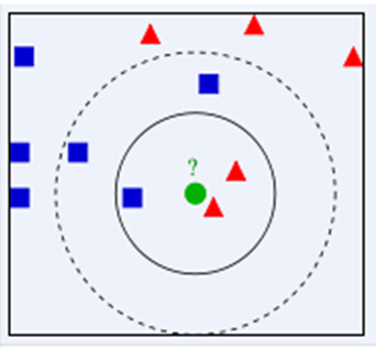
下面通过一个简单的例子说明一下:如下图,绿色圆要被决定赋予哪个类,是红色三角形还是蓝色四方形?如果K=3,由于红色三角形所占比例为2/3,绿色圆将被赋予红色三角形那个类,如果K=5,由于蓝色四方形比例为3/5,因此绿色圆被赋予蓝色四方形类。由此也说明了KNN算法的结果很大程度取决于K的选择。
在KNN中,通过计算对象间距离来作为各个对象之间的非相似性指标,避免了对象之间的匹配问题,在这里距离一般使用欧氏距离或曼哈顿距离。同时,KNN通过依据k个对象中占优的类别进行决策,而不是单一的对象类别决策。这两点就是KNN算法的优势。
接下来对KNN算法的思想总结一下:就是在训练集中数据和标签已知的情况下,输入测试数据,将测试数据的特征与训练集中对应的特征进行相互比较,找到训练集中与之最为相似的前K个数据,则该测试数据对应的类别就是K个数据中出现次数最多的那个分类,其算法的描述为:
1)计算测试数据与各个训练数据之间的距离;
2)按照距离的递增关系进行排序;
3)选取距离最小的K个点;
4)确定前K个点所在类别的出现频率;
5)返回前K个点中出现频率最高的类别作为测试数据的预测分类。
代码实现:
# KNN Regression function
knn <- function(train.data, train.label, test.data, K=3, distance = 'euclidean'){
    ## count number of train samples
    train.len <- nrow(train.data)

    ## count number of test samples
    test.len <- nrow(test.data)

    ## New List for hold the test label (the length is the same with the length of test data)
    test.label <- rep(0,test.len)
    ## calculate distances between samples
    dist <- as.matrix(dist(rbind(test.data, train.data), method= distance))[1:test.len, (test.len+1):(test.len+train.len)]

    ## for each test sample
    for (i in 1:test.len){
        ### find its K nearest neighbours from training sampels...
        nn <- as.data.frame(sort(dist[i,], index.return = TRUE))[1:K,2]

        ### and calculate the predicted labels according to the average of the neighbors’ values
        test.label[i]<-mean(train.label[nn])
    }

    ## return the predict values
    return (test.label)
}

## Load Library
library(ggplot2)
library(reshape2)

## Load Dataset
Task1A_train <- read.csv("Task1A_train.csv")
Task1A_test <- read.csv("Task1A_test.csv")
这里,我们计算error function,直接就是求MSE
距离的话 我们直接用几何距离
## Create train and test data
train.data <- as.matrix(Task1A_train[,1])
train.label <- as.matrix(Task1A_train[,-1])
test.data <- as.matrix(Task1A_test[,1])
test.label <- as.matrix(Task1A_test[,-1])

# KNN Regression function
knn <- function(train.data, train.label, test.data, K=3, distance = 'euclidean'){
    ## count number of train samples
    train.len <- nrow(train.data)

    ## count number of test samples
    test.len <- nrow(test.data)

    ## New List for hold the test label (the length is the same with the length of test data)
    test.label <- rep(0,test.len)
    ## calculate distances between samples
    dist <- as.matrix(dist(rbind(test.data, train.data), method= distance))[1:test.len, (test.len+1):(test.len+train.len)]

    ## for each test sample
    for (i in 1:test.len){
        ### find its K nearest neighbours from training sampels...
        nn <- as.data.frame(sort(dist[i,], index.return = TRUE))[1:K,2]

        ### and calculate the predicted labels according to the average of the neighbors’ values
        test.label[i]<-mean(train.label[nn])
    }

    ## return the predict values
    return (test.label)
}


# calculate the regression error for K in 1:20
# Here we use Mean Square Error (MSE)
miss <- data.frame('K'=1:20, 'train'=rep(0,20), 'test'=rep(0,20)) # New data frame to store the error value
for (k in 1:20){
    miss[k,'train'] <- sum((knn(train.data, train.label, train.data, K=k) - train.label) ^ 2)/nrow(train.data)
    miss[k,'test'] <-  sum((knn(train.data, train.label, test.data, K=k)  - test.label) ^ 2)/nrow(test.data)
}
我们这里采用的是K 从1 到20
那门我们把产生的error给plot出来,大概判断下,哪个K是最小的
## Plot the training and the testing errors versus 1/K for K=1,..,20
miss.m <- melt(miss, id='K') # reshape for visualization
names(miss.m) <- c('K', 'type', 'error')
ggplot(data=miss.m, aes(x=log(1/K), y=error, color=type)) + geom_line() +
       geom_point() +
       scale_color_discrete(guide = guide_legend(title = NULL)) + theme_minimal() +
       ggtitle("KNN Regression Error")
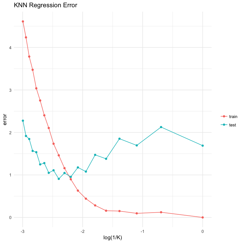
这里我们可以发现 在K= 11的时候,此时针对这个数据集,KNN的在error处理上效果更好。

 浙公网安备 33010602011771号