数据蛙提高-pandas, numpy知识点概括。

Pandas

官方API文档：https://pandas.pydata.org/pandas-docs/stable/reference/index.html

Series和DataFrame数据结构

to_frame(name=None)方法，把Series格式数据转化为DataFrame格式。

索引

使用索引我们就可以对数据进行选取和筛选

使用位置做索引
使用列表做索引
使用切片做索引
使用bool类型索引

loc方法

``.loc[]`` is primarily label based, but may also be used with a boolean array. 主要是基于标签，也可以使用布林数组。

内部参数可以使用单一的标签如1或"a"
一个list或array作为标签，如['a', 'b', 'c']
或切片'a':'f'`，⚠️这是双闭合的,
一个布林数组
一个带单一参数(Series,或DataFrame)的可调用函数并返回验证后的输出结果作为索引。

例子：

df.loc[df["年龄"]>40]

行列的形式：第一个参数是选行，第二个参数选择列

df.loc[[1,2,3], ['年龄', "性别"]]

⚠️第二个参数不能使用整数切片或整数行数。

❌df.loc[0:3, [0,1,2]]
❌df.loc[0:3, 0:2]

iloc方法

``.iloc[]`` is primarily integer position based (from ``0`` to ``length-1`` of the axis), but may also be used with a boolean array.

基于整数位置的，默认0代表第一行或第一列。iloc的字母i就代表integer

可以输入的参数是：

一个整数
一个list,或整数型的array, 如[4, 5]
整数切片， ⚠️左闭合，右开放。
一个布林数组
一个带单一参数(Series,或DataFrame)的可调用函数并返回验证后的输出结果作为索引。

行列的形式：第一个参数是选行，第二个参数选择列。

df.iloc[0:3, 0:2]
等同于
df.iloc[0:3, [0,1,2]]

⚠️只能用整数。不能使用具体的列名字。

MultiIndex 多级索引

A multi-level, or hierarchical, index object for pandas objects. 一种多级别，或多层的Pandas索引对象。

pd.MultiIndex.from_arrays() 把一个数组转换为一个多级索引。

例子：

idx = pd.MultiIndex.from_arrays([
    ['warm', 'warm', 'cold', 'cold'],
    ['dog', 'falcon', 'fish', 'spider']],
    names=['blooded', 'animal'])

#产生2层索引：
MultiIndex([('warm',    'dog'),
            ('warm', 'falcon'),
            ('cold',   'fish'),
            ('cold', 'spider')],
           names=['blooded', 'animal'])

使用idx创建一个Series:

s = pd.Series([4, 2, 0, 8], name='legs', index=idx)

blooded  animal
warm     dog       4
         falcon    2
cold     fish      0
         spider    8
Name: legs, dtype: int64

s的索引有2级。0和1级别。

⚠️使用sum(level=0)计算第0级的数据之和：（本质就是按照level=0分组，然后求分组后的和。）

s.sum(level=0)
#得到：
blooded
warm    6
cold    8
dtype: int64

⚠️，得到索引层的数量：

s.index.nlevels
#2

判断是否是按照字典的结构排列：

s.index.is_lexsorted()

Series.unstack(level=0) ->DataFrame, Unstacked Series

解堆。把有多重索引的Series,或piovt_table拆解成DataFrame

其他

MultiIndex.from_product(iterables)　　

Create a MultiIndex from the cartesian product of iterables.用可迭代对象创建一个MultiIndex对象。

numbers = [0, 1, 2]
colors = ['green', 'purple']
pd.MultiIndex.from_product([numbers, colors],
                           names=['number', 'color'])
#产生类似笛卡尔积的list集合.
MultiIndex([(0,  'green'),
            (0, 'purple'),
            (1,  'green'),
            (1, 'purple'),
            (2,  'green'),
            (2, 'purple')],
           names=['number', 'color'])

MultiIndex.from_tuples

multiIndex.from_frame

一道练习题：

letters = ['A', 'B', 'C']
numbers = list(range(10))
#生成一个MultiIndex:
x = pd.MultiIndex.from_product([letters, numbers], names = ['leters', 'numbers'])
s = pd.Series(np.random.rand(30), index = x)

判断index是否是lexcon即字典排序模式：is_lexsorted()

s.index.is_lexsorted()

查询：

#查询所有的索引是1，2，6的记录：
s.loc[:, [1,2,6]]
#查询level0，从开始到"B",然后选出level1,从5到结束：
s.loc[:"B", 5:]

求和：

s.sum(level=0)

unstack()

把MultiIndex转换为普通的DataFrame:

s.unstack().

swaplevel(0,1)

交换多重索引的顺序

n = s.swaplevel(0,1)
n.index.is_lexsorted()  #False
n.sort_index() #重新整理。笛卡尔积

DataFrame的常用方法

计算函数： max, min, sum
更改索引(index, columns)名字: rename
排序 sort_values()
值替换 replace()
df.age.unique()得到age列的唯一值，array格式。
df.age.value_counts()，按照age进行分组统计counts
累加求和 cumulative sum简写为： cumsum
增加、删除多种方法，

drop函数既可以删除行也可以删除列。
del df['列名']. 删除列。
使用map函数修改一列的值。df.sex = df['sex'].map({'男':'female','女':'male'})

矩阵运算: 可以加减乘除。
df.idxmax()获得每列最大值的id.

sqlalchemy是一个orm：

create_engine() 创建一个连接到具体某个数据库的对象。
pandas的方法to_sql和read_sql

相关知识见之前的博客：Python3 MySQL 数据库连接

连接和分组：

pd.concat(),
pd.merge()
pd.列名.value_counts()，得到一个列每个数据有多少个。
groups = df.groupby('列名')
相关方法groups.size(), groups.groups
可以使用for x in groups: 即groups是可迭代对象。
groups.mean()/sum()等计算函数。

聚合：

使用aggregate()函数, agg是别名。例子：

grouped.aggregate(['std', 'sum'])
grouped.agg({"age":[np.mean, np.sum],"vip_buy_times":np.sum}) #不同列不同聚合函数
或者用grouped.agg({"age": "mean", "visits": "sum"}) 这种字符串方式。

转换过滤：

df.fillna(0)把表格中的NaN改为用0表示。
transform函数：

groups.age.transform(lambda x : x + 100)

groups.filter()过滤数据

一些方法详解：

Groupby对象

GroupBy对象是pandas.DataFrame.groupby(), pandas.Series.groupby()调用的返回值。

GroupBy.count():计算每列的统计数，不包括NaN.

SeriesGroupby.nlargest(3)

返回分组后的Series的前3个最大值。

df = pd.DataFrame({'grps': list('aaabbcaabcccbbc'), 
                   'vals': [12,345,3,1,45,14,4,52,54,23,235,21,57,3,87]})

df = df.groupby("grps")['vals'].nlargest(3)
#结果：按照grps分组后，vals列的前3个最大的值。
grps    
a     1     345
      7      52
      0      12
b     12     57
      8      54
      4      45
c     10    235
      14     87
      9      23
Name: vals, dtype: int64

pandas.pivot_table(data, ...后面参数一样)

pandas.DataFrame.pivot_table(self, values=None, index=None, columns=None, aggfunc="mean")

返回DataFrame, 一个EXcel样式的pivot table。

对index指定的列分纵向组，然后根据columns指定的列横向组。用values指定的列填充数据，用aggfunc来使用计算函数。

具体点击链接看案例。

pandas.Series.shift(self. periods=1) DataFrame也可以使用。

整个数据表向下移动一行。具体看案例。

pandas.DataFrame.drop_duplicates（self, subset=None, keep='first', inplace=False）

返回的DataFrame去掉了重复的行。

subset：可以是column label或sequence of labels, 其他。默认作用于所有的列。可以设置,如

df = pd.DataFrame({'A': [1, 2, 2, 3, 4, 5, 5, 5, 6, 7, 7]})
# 整个列去重, 生成新的DataFrame：
df1 = df.drop_duplicates(subset='A')

对应的还有一个方法：

duplicated(subset=None, keep='first')

keep参数即保留第一个，还可以选择last(保留最后一个), False(都移除)

DataFrame.sub(self, other, axis="columns") 减法，

还有add, div，mul, 可以使用+-*/符号。

Pandas.cut(x, bins)

https://pandas.pydata.org/pandas-docs/stable/search.html?q=groupby#

参数：

x: array-like输入的数组，用于binned。只能是一维的。

bins: int, sequence of scalars or IntervalIndex。

pd.cut()的作用，有点类似给成绩设定优良中差，比如：0-59分为差，60-70分为中，71-80分为优秀等等，在pandas中，也提供了这样一个方法来处理这些事儿

pd.cut(np.array([1, 7, 5, 4, 6, 3]), 3)
#输出：
[(0.994, 3.0], (5.0, 7.0], (3.0, 5.0], (3.0, 5.0], (5.0, 7.0], (0.994, 3.0]]
Categories (3, interval[float64]): [(0.994, 3.0] < (3.0, 5.0] < (5.0, 7.0]]

参考这篇文章：https://blog.csdn.net/missyougoon/article/details/83986511

Time series and DatetimeIndex

pandas is fantastic for working with dates and times. Pandas包括了大量功能来处理time series data。

⚠️这是一个非常大的功能模块，内容非常多

pd.to_datetime()

可以把np.datetime64, pd的datetime数据结构，字符串'1/1/2018'转换为pd的DatetimeIndex格式。

import datetime
dti = pd.to_datetime(['1/1/2018', np.datetime64('2018-01-01'),datetime.datetime(2018, 1, 1)])

DatetimeIndex(['2018-01-01', '2018-01-01', '2018-01-01'], dtype='datetime64[ns]', freq=None)

date_range(start=None, end=None, periods=None,freq=None)

start: str or datetime-like, optional

Left bound for generating dates.

end: str or datetime-like, optional

Right bound for generating dates.

periods: int, optional

Number of periods to generate.

freq: str or DateOffset, default ‘D’ 即，daily frequency，

Frequency strings can have multiples, e.g. ‘5H’.
⚠️ freq有非常多的显示方式：具体见 here ！！！

4个参数，freq默认是D。 start必须指定， end或periods至少指定一个。

pd.date_range(start='1/1/2018', periods=8)
#结果：
DatetimeIndex(['2018-01-01', '2018-01-02', '2018-01-03', '2018-01-04',
               '2018-01-05', '2018-01-06', '2018-01-07', '2018-01-08'],
              dtype='datetime64[ns]', freq='D')

Resampling()

sample，动词：抽查样本。resampling。

resampling()方法是基于time的分组操作groupby，后面跟随一个reduction方法，作用于它的每个组。

例子：

# freq="min"重复级别是分钟。从2012-1-1开始，每分钟一个数据，一天有1440个分钟。
rng = pd.date_range('1/1/2012', periods=1440, freq='min') 
# 生成Series
s = pd.Series(np.random.randint(0, 500, len(rng)), index=rng)
# 
s.resample('120Min').sum()

生成：（每2个小时内的数字的和，按照每2个小时进行分组！）

2012-01-01 00:00:00    27807
2012-01-01 02:00:00    32306
2012-01-01 04:00:00    31818
2012-01-01 06:00:00    31658
2012-01-01 08:00:00    32170
2012-01-01 10:00:00    32313
2012-01-01 12:00:00    29606
2012-01-01 14:00:00    32071
2012-01-01 16:00:00    30189
2012-01-01 18:00:00    30546
2012-01-01 20:00:00    29621
2012-01-01 22:00:00    31779
Freq: 120T, dtype: int64

numpy的使用

NumPy（Numerical Python的简称）是Python科学计算的基础包。实际应用中用的不多。

官网教程：https://numpy.org/doc/1.18/user/index.html

1. numpy 的介绍和数据类型: nmupy.ndarray，这个数据中的元素类型是一样的：

大致类型是浮点数、复数、整数、布尔值、字符串，还是普通的Python对象
如果处理大数据，需要知道数据储存方式：：一个类型名（如 float或int），后面跟一个用于表示各元素位长的数字

2. 创建 array 以及从已有数据创建 zeros，ones，empty, full, eye 函数

>>> np.zeros( (3,4) )
array([[ 0.,  0.,  0.,  0.],
       [ 0.,  0.,  0.,  0.],
       [ 0.,  0.,  0.,  0.]])
>>> np.ones( (2,3,4), dtype=np.int16 )                # dtype can also be specified
array([[[ 1, 1, 1, 1],
        [ 1, 1, 1, 1],
        [ 1, 1, 1, 1]],
       [[ 1, 1, 1, 1],
        [ 1, 1, 1, 1],
        [ 1, 1, 1, 1]]], dtype=int16)
>>> np.empty( (2,3) )                                 # uninitialized, output may vary
array([[  3.73603959e-262,   6.02658058e-154,   6.55490914e-260],
       [  5.30498948e-313,   3.14673309e-307,   1.00000000e+000]])
>>> np.full((2,2), 12). #填充数值12.

*_like()

a.shape
#(5,)
np.zeros_like(a)
#array([0, 0, 0, 0, 0])
#*_like接受一个参数，是array_like的shape。有empty_like, full_like, onse_like

np.eye()

其实是identity的谐音。第一个参数，代表2维数组的对角线长度，值为1，其他值为0

np.eye(3)
#
array([[1., 0., 0.],
       [0., 1., 0.],
       [0., 0., 1.]])

3.

numpy.arange(start, stop, step, dtype), 返回ndarray
numpy.reshape,
numpy.random.random(),
numpy.linspace() 类似arange
numpy.sin()

4. numpy 的切片和索引, 分为一维和多维。

⚠️nump的切片比较特殊，它产生一个指针指向原内存地址位置的数据片段。因此对切片修改，就会作用于原数组。这是因为numpy用于大数据计算。为了效率不适合来回的复制。
⚠️numpy的切片，左闭右开，ndarray[1:3] 会返回第2行和第3行，即索引为1和2的行。
花式索引：比较特别的索引。下面是一个例子：

arr = np.arange(32).reshape((8,4))
arr
array([[ 0,  1,  2,  3],
       [ 4,  5,  6,  7],
       [ 8,  9, 10, 11],
       [12, 13, 14, 15],
       [16, 17, 18, 19],
       [20, 21, 22, 23],
       [24, 25, 26, 27],
       [28, 29, 30, 31]])

arr[[1,5,7,2], [0,3,1,2]] #结果可能和你想的不一样！⚠️ 答案：array([ 4, 23, 29, 10])

这是因为第2个参数[0,3,1,2] 中的每个元素不代表取整列。

arr[[1,5,7,2], [0,3,1,2]] 是，从arr中取得(1, 0)，（5，3）（7，1）（2，2）的4个值。

原先我们想得到整列的数据，可以这么写：

 arr[[1, 5, 7, 2]][:, [0, 3, 1, 2]]

5. bool 索引以及数组索引。

大小相同的ndarray会进行比较。生成布尔值数组。
arr > 4 返回值为bool的数组。

a = array([[ 1,  2,  3,  4],
       [ 5,  6,  7,  8],
       [ 9, 10, 11, 12]])

a > 4
#
#array([[False, False, False, False],
#       [ True,  True,  True,  True],
#       [ True,  True,  True,  True]])

a[a>4]
#array([ 5,  6,  7,  8,  9, 10, 11, 12])

6. 数值转换ndarray。transpose转换位置: 行变为列，列变为行。

np.transpose(arr)等同于arr.T

主要用在矩阵乘积计算Matrix multiplication

定义：如果矩阵A是m*n，矩阵B是n*p，那么A*B会是一个m*P矩阵，也叫做一般矩阵乘积

有2种计算方法：

由定义公式计算。
向量方法：把向量和各系数相乘后相加起来。

${\begin{bmatrix}1&0&2\\-1&3&1\end{bmatrix}}\cdot {\begin{bmatrix}3&1\\2&1\\1&0\end{bmatrix}}={\begin{bmatrix}1{\begin{bmatrix}3&1\end{bmatrix}}+0{\begin{bmatrix}2&1\end{bmatrix}}+2{\begin{bmatrix}1&0\end{bmatrix}}\\-1{\begin{bmatrix}3&1\end{bmatrix}}+3{\begin{bmatrix}2&1\end{bmatrix}}+1{\begin{bmatrix}1&0\end{bmatrix}}\end{bmatrix}}={\begin{bmatrix}{\begin{bmatrix}3&1\end{bmatrix}}+{\begin{bmatrix}0&0\end{bmatrix}}+{\begin{bmatrix}2&0\end{bmatrix}}\\{\begin{bmatrix}-3&-1\end{bmatrix}}+{\begin{bmatrix}6&3\end{bmatrix}}+{\begin{bmatrix}1&0\end{bmatrix}}\end{bmatrix}}$ $={\begin{bmatrix}5&1\\4&2\end{bmatrix}}$

3. 向量表方法：行向量和列向量的内积：

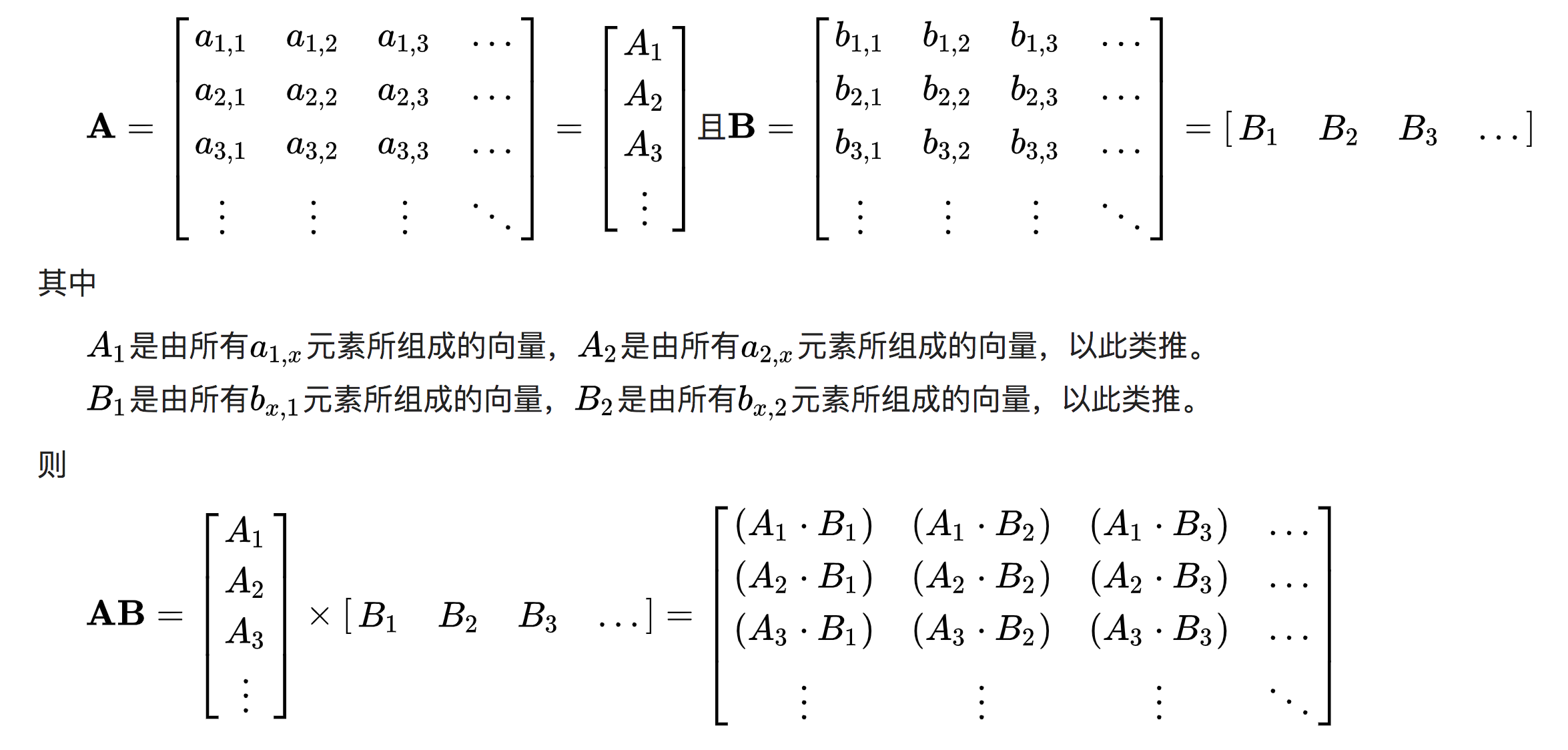
实例：

arr = np.random.randint(1,10, (2,2))
array([[5, 1],
       [3, 7]])
arr1 = arr.T
array([[5, 3],
       [1, 7]])

那么用方法3，arr的每行✖️arr1的每列：

np.dot(arr, arr1)
#array([[26, 22],
#      [22, 58]])

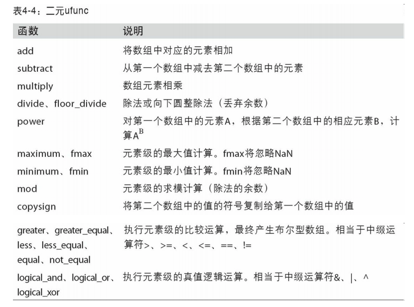
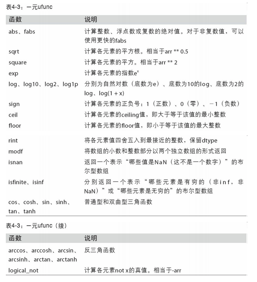
通用函数，uFunc

是一种对ndarray中的数据执行元素级运算的函数。

dtype.astype(dtype) 类型转换
np.sum()求和。可以使用axis在index, columns方向上求和。
np.argmax(), 求最大值的索引。
求指数。np.exp(x) ,等价的写为e^x，e即exponent幂数，近似等于 2.718281828，还称为欧拉数。
np. sqrt(x), Return the non-negative square-root of an array返回非负平方根的数组。
改变2维数组的形状，产生一个新的数组：
- dtype.ravel() 多维变一维
- dtype.reshape(2,3) 改变数组的形状。
- a.T，行变列，列变行。
- ⚠️，dtype.reshape(3, -1) 中的-1，这个参数数值的作用是自动计算：根据原数组，我设置一个行为3，但列让numpy自动计算列的长度。
np.tile(A, repeat), 把数组A，重复输出repeat次， repeat可以是多维的。tile瓷砖地砖。

a = np.arange(0,40,10) b = np.tile(a, (2,2)) #输出 array([[ 0, 10, 20, 30, 0, 10, 20, 30], [ 0, 10, 20, 30, 0, 10, 20, 30]])

np.floor(a), 返回数据a的floor， 1.5的floor是1，-0.5的floor是-1。

矩阵array的拼接：

np.hstack((array1, array2)) 水平方向上把2个数组拼接
np.vstack((array1, array2)) 垂直方向上把2个数组拼接

矩阵array的分割：

np.hsplit(array1, 3) 水平方向上把数组分出3等份。
np.vsplit(array2, 2) 垂直方向上把数组分成2份

4.3 利用数组进行数据处理

用数组表达式代替循环的做法，通常被称为矢量化。一般来说，矢量化数组运算要比等价的纯Python方式快上一两个数量级（甚至更多），尤其是各种数值计算。

将条件逻辑表述为数组运算：np.where(condition, x, y)

本质就是条件判断，if condition: x else: y

数学和统计方法

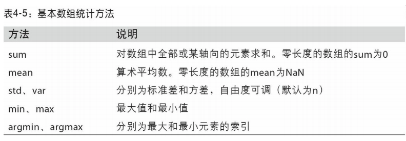
np.argsort():

返回的是未排序时数组的索引。(默认行方向)
是np.sort()的补充。返回np.sort()后得到的排序数组中，元素在未排序时的索引。

用于布尔型数组的方法

any用于测试数组中是否存在一个或多个True，
all则检查数组中所有值是否都是True：

⚠️两个shape形状一样的数组可以进行四则运算。可以使用+-*/。也可以使用函数：add, subtract, multiply, divide.

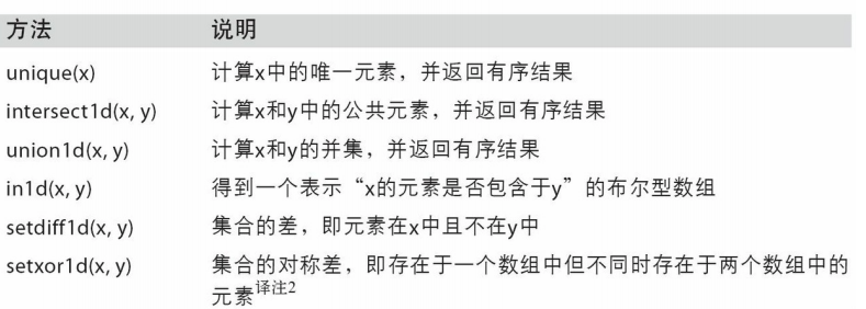
唯一化以及其它的集合逻辑

4.5 线性代数

线性代数（如矩阵乘法、矩阵分解、行列式以及其他方阵数学等）是任何数组库的重要组成部分。

NumPy提供了一个用于矩阵乘法的 dot函数（既是一个数组方法也是numpy命名空间中的一个函数）

本文上面已经提到。

x @ np.ones(3) #这里@相当于dot函数

4.6 伪随机数生成 np.random

在概率论和数据挖掘中用到。官方主页RANDOM:https://docs.scipy.org/doc/numpy/reference/random/index.html

rand(d0, d1, ..., dn) Random values in a given shape. 在[0, 1)范围内返回浮点数。
randn(d0, d1, ..., dn) Return a sample (or samples) from the “standard normal” distribution. 返回符合正态分布的样本数据。
randint(low[, high, size, dtype]) Return random integers from low (inclusive) to high (exclusive). 返回从low到high之间的数，shape是size参数定义的。
random([size]) Return random floats in the half-open interval [0.0, 1.0).
choice(a[, size, replace=True]) Generates a random sample from a given 1-D array

4.7 示例：随机漫步（《利用pandas》135页）

通过模拟随机漫步来说明如何运用数组运算

matplotlib

一个Pandas内置的绘图库。

Pandas is highly integrated with the plotting library matplotlib, and makes plotting DataFrames very user-friendly! Plotting in a notebook environment usually makes use of the following boilerplate:

import matplotlib.pyplot as plt
%matplotlib inline
plt.style.use('ggplot')

pyplot是一个制图对象。
第2行不弹出新窗口
一种显示风格。

`DataFrame.plot`(self, *args, **kwargs)

参数：

数据是DataFrame/ Series
x是label或position,默认None
类型：有多种，比如scatter散点图, bar垂直条
很多参数。

例子：绘制散点图：

df = pd.DataFrame({"xs":[1,5,2,8,1], "ys":[4,2,1,9,6]})

df.plot.scatter("xs", "ys", color = "red", marker = "x")

pandas.DataFrame.plot.scatter(self, x, y, s=None, c=None, **kwargs)

x: int or str 横轴的名字，位置
y: int or str 纵轴的名字，位置
c：代表点的颜色，可以是单一的，也可以是一个sequence.
s: scalar or array_like，每个点的大小。

数据清洗

详细知识点见博客：https://www.cnblogs.com/chentianwei/p/12322459.html

It happens all the time: someone gives you data containing malformed strings, Python, lists and missing data. How do you tidy it up so you can get on with the analysis?

把一些数据中包含的糟糕字符串，Python,列表，缺失数据进行处理，以便分析。

DataFrame.interpolate(self, method="linear", axis=0) 插入数据。

根据传入的方法来调整数据。默认是linear, 忽视index，让数据equally spaced。

"pad": 填充NaNs，使用上一行的已经存在的值。

参数limit: 填充NaNs的最大次数。值必须大于0.

s = pd.Series([0, 1, np.nan, 3])
s
0    0.0
1    1.0
2    NaN
3    3.0
dtype: float64
s.interpolate()
0    0.0
1    1.0
2    2.0
3    3.0
dtype: float64

把一列数据，字符串格式，分裂成两列。

#From_to是列名，从一个地区到另一个地区，因此要分成两列。
temp = df.From_To.str.split('_', expand=True)
#再赋予列名
temp.columns = ["From", "To"]

str的方法：

split()

posted @ 2020-02-06 11:02 Mr-chen 阅读(615) 评论(0) 编辑收藏举报

会员力量，点亮园子希望

刷新页面返回顶部

Mr-chen