01笔记
6. flat, stack(),
7. export_graphviz()
8. Pipeline() 函数
9. 画图
10.正确率
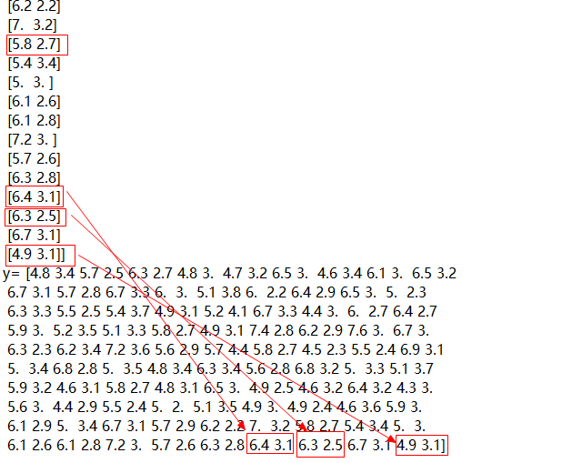
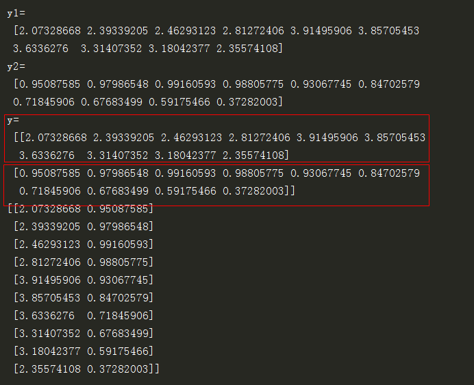
11.过拟合 12 np.vstack((y1, y2)) 将两组数据拼接到一个二元数组
import numpy as np
from sklearn import svm
from sklearn.model_selection import train_test_split
import matplotlib as mpl
import matplotlib.pyplot as plt
2.导入数据
path = '8.iris.data'
data = np.loadtxt(path, dtype=float, delimiter=',', converters={4: iris_type}) #delimiter:分隔样本,converters用于提供缺失数据的默认值
path = '8.iris.data'
data = np.loadtxt(path, dtype=float, delimiter=',', converters={4: iris_type}) #delimiter:分隔样本,converters用于提供缺失数据的默认值
3.获取x,y的值
x, y = np.split(data, (4,), axis=1) # axis=1,则沿着 列方向取值,x取前4列,所有行;y取其余所有列,
x = x[:, :2] #2. 两列数据,即两个特征
x = x[:, :2] #2. 两列数据,即两个特征
注: x, y = np.split(data, (4,), axis=0) # axis=0,则沿着 行方向取值,x取前4行,所有列;y取其余所有行
4. 利用x,y得到相应的训练集和测试集
x_train, x_test, y_train, y_test = train_test_split(x, y, random_state=1, train_size=0.6)
5. x_train, x_train.ravel()的结果如下:x_train.ravel() 作用: 取x_train 样本值的每一行,并将其合并成一个大行
6. flat, stack(),

# 画图
N, M = 100, 100 # 横纵各采样多少个值
x1_min, x1_max = x[:, 0].min(), x[:, 0].max() # 第0列的范围,最小最大值
x2_min, x2_max = x[:, 1].min(), x[:, 1].max() # 第1列的范围,最小最大值
t1 = np.linspace(x1_min, x1_max, N) # 从4.3到7.9之间产生100个等差分布的样本点
t2 = np.linspace(x2_min, x2_max, M)
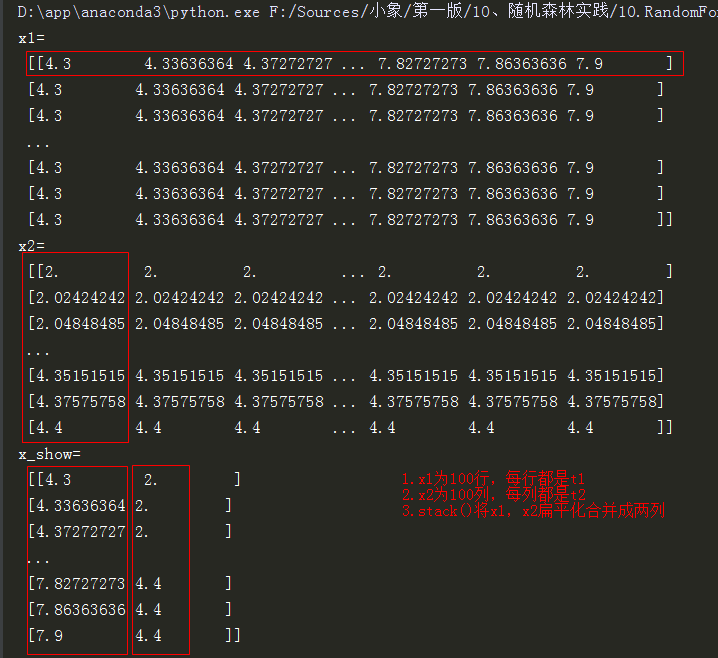
x1, x2 = np.meshgrid(t1, t2) # 生成网格采样点。x1:生成相同的100行,每行都是t1;x2生成相同的100列,每列都是t2
# print('x1.flat=',x1.flat) # x1.flat输出结果= <numpy.flatiter object at 0x000000000C75B450>
x_show = np.stack((x1.flat, x2.flat), axis=1) # 测试点。x1,x2都扁平化,取x1的行和x2的列,合并成两列
print('x_show=',x_show)
7. export_graphviz()
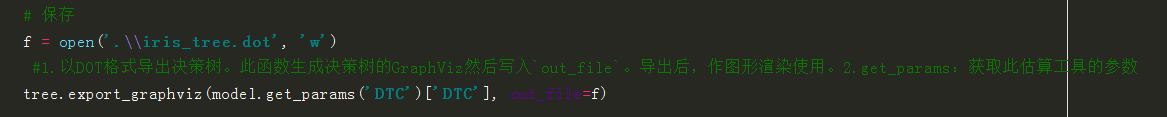
    # 保存
    f = open('.\\iris_tree.dot', 'w')
     #1.以DOT格式导出决策树。此函数生成决策树的GraphViz然后写入`out_file`。导出后,作图形渲染使用。2.get_params:获取此估算工具的参数
    tree.export_graphviz(model.get_params('DTC')['DTC'], out_file=f)
8. Pipeline() 函数

    # 决策树参数估计
    # min_samples_split = 10:如果该结点包含的样本数目大于10,则(有可能)对其分支
    # min_samples_leaf  = 10:若将某结点分支后,得到的每个子结点样本数目都大于10,则完成分支;否则,不进行分支
    model = Pipeline([
        ('ss', StandardScaler()),
        ('DTC', DecisionTreeClassifier(criterion='entropy', max_depth=3))]) # max_depth数值可以更改,但要预防过拟合
    # clf = DecisionTreeClassifier(criterion='entropy', max_depth=3)
    model = model.fit(x_train, y_train)
    y_test_hat = model.predict(x_test)              # 测试数据
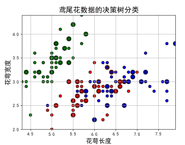
9. 画图
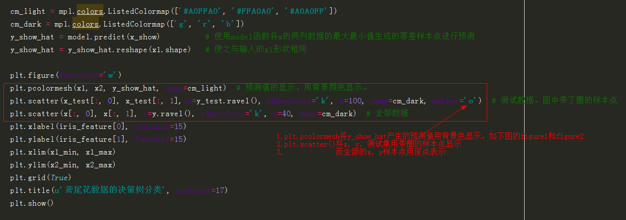
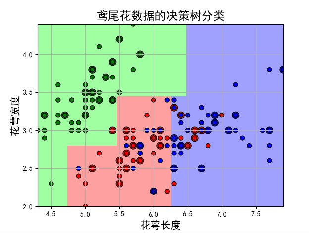
    cm_light = mpl.colors.ListedColormap(['#A0FFA0', '#FFA0A0', '#A0A0FF'])
    cm_dark = mpl.colors.ListedColormap(['g', 'r', 'b'])
    y_show_hat = model.predict(x_show)          # 使用model函数将x的两列数据的最大最小值生成的等差样本点进行预测
    y_show_hat = y_show_hat.reshape(x1.shape)   # 使之与输入的x1形状相同

    plt.figure(facecolor='w')
    plt.pcolormesh(x1, x2, y_show_hat, cmap=cm_light)  # 预测值的显示。用背景颜色显示。
    plt.scatter(x_test[:, 0], x_test[:, 1], c=y_test.ravel(), edgecolors='k', s=100, cmap=cm_dark, marker='o')  # 测试数据。图中带了圈的样本点
    plt.scatter(x[:, 0], x[:, 1], c=y.ravel(), edgecolors='k', s=40, cmap=cm_dark)  # 全部数据
    plt.xlabel(iris_feature[0], fontsize=15)
    plt.ylabel(iris_feature[1], fontsize=15)
    plt.xlim(x1_min, x1_max)
    plt.ylim(x2_min, x2_max)
    plt.grid(True)
    plt.title(u'鸢尾花数据的决策树分类', fontsize=17)
    plt.show()
10 正确率
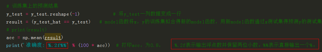
    # 训练集上的预测结果
    y_test = y_test.reshape(-1)            # 将y_test一列数据变成一行
    result = (y_test_hat == y_test)   # model函数将x,y的训练集进行拟合得到新的model函数,再用新model函数通过x的测试集来预测y的测试集,True则预测正确,False则预测错误
    # print(result)
    acc = np.mean(result)
    print('准确度: %.2f%%' % (100 * acc))  # 打印acc,为0.8,    %.2f表示输出浮点数并保留两位小数。%%表示直接输出一个%。
11. 过拟合


   # 过拟合:错误率
    depth = np.arange(1, 15)
    err_list = []
    for d in depth:
        clf = DecisionTreeClassifier(criterion='entropy', max_depth=d)
        clf = clf.fit(x_train, y_train)         # 决策树分类函数进行拟合
        y_test_hat1 = clf.predict(x_test)       # 用新的拟合函数通过x的测试集进行预测出y的测试集。测试数据
        result = (y_test_hat1 == y_test)        # 预测出y的测试集与y原本的测试集对比。True则预测正确,False则预测错误
        err = 1 - np.mean(result)
        err_list.append(err)
        print(d, ' 准确度: %.2f%%' % (100 * err))
    plt.figure(facecolor='w')
    plt.plot(depth, err_list, 'ro-', lw=2)
    plt.xlabel(u'决策树深度', fontsize=15)
    plt.ylabel(u'错误率', fontsize=15)
    plt.title(u'决策树深度与过拟合', fontsize=17)
    plt.grid(True)
    plt.show()
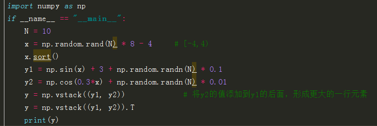
12 np.vstack((y1, y2)) 将两组数据拼接到一个二元数组

 浙公网安备 33010602011771号