扩散模型的推导
主要是根据以下网址学习diffusion的数学形式:网址
首先使用\(q\)表示前向扩散过程,使用\(p\)表示逆向过程。
\[q(\mathbf{x}_t|\mathbf{x}_{t-1})=\mathcal{N}(\mathbf{x}_t;\sqrt{1-\beta}_t\mathbf{x}_{t-1},\beta_t\mathbf{I})\quad q(\mathbf{x}_{1:T}|\mathbf{x}_0)=\prod_{t=1}^Tq(\mathbf{x}_t|\mathbf{x}_{t-1})
\]
当\(\beta_t\)较小的时候,逆向过程也可以认为是一个高斯分布:
\[p_\theta(\mathbf{x}_{0:T})=p(\mathbf{x}_T)\prod_{t=1}^Tp_\theta(\mathbf{x}_{t-1}|\mathbf{x}_t)\quad p_\theta(\mathbf{x}_{t-1}|\mathbf{x}_t)=\mathcal{N}(\mathbf{x}_{t-1};\boldsymbol{\mu}_\theta(\mathbf{x}_t,t),\boldsymbol{\Sigma}_\theta(\mathbf{x}_t,t))
\]
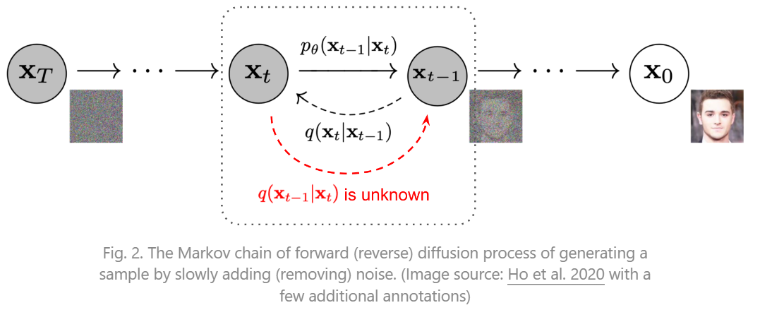
前向添加噪声的过程是一个马尔科夫链,\(t\)时刻添加噪声的图像只和\(t-1\)时刻有关。
令\(\alpha_{t}=1-\beta_{t}\quad,\bar{\alpha}_{t}=\prod_{i=1}^{t}\alpha_{i}\mathrm{:}\)
在前向过程中添加高斯噪声:
\[\begin{aligned}
\mathbf{x}_{t}& =\sqrt{\alpha_t}\mathbf{x}_{t-1}+\sqrt{1-\alpha_t}\boldsymbol{\epsilon}_{t-1} \\
&=\sqrt{\alpha_t\alpha_{t-1}}\mathbf{x}_{t-2}+\sqrt{1-\alpha_t\alpha_{t-1}}\bar{\boldsymbol{\epsilon}}_{t-2} \\
&=\ldots \\
&=\sqrt{\bar{\alpha}_t}\mathbf{x}_0+\sqrt{1-\bar{\alpha}_t}\boldsymbol{\epsilon} \\
从而得到:\\
q(\mathbf{x}_t|\mathbf{x}_0)& =\mathcal{N}(\mathbf{x}_t;\sqrt{\bar{\alpha}_t}\mathbf{x}_0,(1-\bar{\alpha}_t)\mathbf{I})
\end{aligned}
\]
我们需要根据前向过程求得逆向过程的分布情况,即求得如下的分布情况(我们已经根据一些前置知识知道它是正态分布,所以只用求取如下的参数):
\[q(\mathbf{x}_{t-1}|\mathbf{x}_t,\mathbf{x}_0)=\mathcal{N}(\mathbf{x}_{t-1};\tilde{\color{blue}{\boldsymbol{\mu}}(\mathbf{x}_t,\mathbf{x}_0)},\color{red}{\tilde{\boldsymbol{\beta}}_t}\mathbf{I})
\]
根据贝叶斯公式:
\[\begin{aligned}
q(\mathbf{x}_{t-1}|\mathbf{x}_t,\mathbf{x}_0)& =q(\mathbf{x}_t|\mathbf{x}_{t-1},\mathbf{x}_0)\frac{q(\mathbf{x}_{t-1}|\mathbf{x}_0)}{q(\mathbf{x}_t|\mathbf{x}_0)} \\
&\propto\exp\left(-\frac12(\frac{(\mathbf{x}_t-\sqrt{\alpha_t}\mathbf{x}_{t-1})^2}{\beta_t}+\frac{(\mathbf{x}_{t-1}-\sqrt{\bar{\alpha}_{t-1}}\mathbf{x}_0)^2}{1-\bar{\alpha}_{t-1}}-\frac{(\mathbf{x}_t-\sqrt{\bar{\alpha}_t}\mathbf{x}_0)^2}{1-\bar{\alpha}_t})\right) \\
&=\exp\left(-\frac12(\frac{\mathbf{x}_t^2-2\sqrt{\alpha_t}\mathbf{x}_t\mathbf{x}_{t-1}+\alpha_t\mathbf{x}_{t-1}^2}{\beta_t}+\frac{\mathbf{x}_{t-1}^2-2\sqrt{\bar{\alpha}_{t-1}}\mathbf{x}_0\mathbf{x}_{t-1}+\bar{\alpha}_{t-1}\mathbf{x}_0^2}{1-\bar{\alpha}_{t-1}}-\frac{(\mathbf{x}_t-\sqrt{\bar{\alpha}_t}\mathbf{x}_0)^2}{1-\bar{\alpha}_t})\right) \\
&=\exp\left(-\frac12\color{red}{((\frac{\alpha_t}{\beta_t}+\frac1{1-\bar{\alpha}_{t-1}})x_{t-1}^2}-\color{blue}{(\frac{2\sqrt{\alpha_t}}{\beta_t}x_t+\frac{2\sqrt{\alpha}_{t-1}}{1-\bar{\alpha}_{t-1}}x_0)x_{t-1}}+\color{black}{C(x_t,x_0)}\right)
\end{aligned}
\]
根据正太分布的公式:
\[\begin{aligned}
f(x) &= \frac{1}{{\sigma \sqrt{{2\pi}}}} e^{-\frac{1}{2}\left(\frac{{x-\mu}}{{\sigma}}\right)^2}\\
&= \frac{1}{{\sigma \sqrt{{2\pi}}}} \exp\left(-\frac{1}{2}\left(\frac{{x^2-2\mu x+\mu^2}}{{\sigma^2}}\right)\right)\\
\end{aligned}
\]
从而可以求解出\(\tilde{\boldsymbol{\beta}}_t\)和\(\tilde{\boldsymbol{\mu}}(\mathbf{x}_t,\mathbf{x}_0)\):
\[\begin{aligned}
\tilde{\beta}_{t}& =1/(\frac{\alpha_t}{\beta_t}+\frac1{1-\bar{\alpha}_{t-1}})=1/(\frac{\alpha_t-\bar{\alpha}_t+\beta_t}{\beta_t(1-\bar{\alpha}_{t-1})})=\color{red}{\frac{1-\bar{\alpha}_{t-1}}{1-\bar{\alpha}_t}\cdot\beta_t} \\
\tilde{\boldsymbol{\mu}}_t(\mathbf{x}_t,\mathbf{x}_0)& =(\frac{\sqrt{\alpha_t}}{\beta_t}\mathbf{x}_t+\frac{\sqrt{\bar{\alpha}_{t-1}}}{1-\bar{\alpha}_{t-1}}\mathbf{x}_0)/(\frac{\alpha_t}{\beta_t}+\frac1{1-\bar{\alpha}_{t-1}}) \\
&=(\frac{\sqrt{\alpha_t}}{\beta_t}\mathbf{x}_t+\frac{\sqrt{\bar{\alpha}_{t-1}}}{1-\bar{\alpha}_{t-1}}\mathbf{x}_0)\frac{1-\bar{\alpha}_{t-1}}{1-\bar{\alpha}_t}\cdot\beta_t \\
&=\color{red}{\frac{\sqrt{\alpha_t}(1-\bar{\alpha}_{t-1})}{1-\bar{\alpha}_t}\mathbf{x}_t+\frac{\sqrt{\bar{\alpha}_{t-1}}\beta_t}{1-\bar{\alpha}_t}\mathbf{x}_0}
\end{aligned}
\]
根据上述\(\bold{x}_0,\bold{x_t}\)关系,将\(\tilde{\boldsymbol{\mu}}(\mathbf{x}_t,\mathbf{x}_0)\)表示:
\[\begin{aligned}
\tilde{\boldsymbol{\mu}}_t& =\frac{\sqrt{\alpha_t}(1-\bar{\alpha}_{t-1})}{1-\bar{\alpha}_t}\mathbf{x}_t+\frac{\sqrt{\bar{\alpha}_{t-1}}\beta_t}{1-\bar{\alpha}_t}\frac1{\sqrt{\bar{\alpha}_t}}(\mathbf{x}_t-\sqrt{1-\bar{\alpha}_t}\boldsymbol{\epsilon}_t) \\
&=\color{red}{\frac1{\sqrt{\alpha_t}}\left(\mathrm{x}_t-\frac{1-\alpha_t}{\sqrt{1-\bar{\alpha}_t}}\epsilon_t\right)}
\end{aligned}
\]
扩散模型现在需要的就是通过一个网络来预测\(\tilde{\boldsymbol{\mu}}(\mathbf{x}_t,\mathbf{x}_0)\),如果我们得到了很好的\(\tilde{\boldsymbol{\mu}}(\mathbf{x}_t,\mathbf{x}_0)\)参数,那么我们可以能够得到逆向采样过程的分布,通过不断地进行采样,就可以生成逆向采样过程的图像了。
我们需要设计网络来预测,那么我们就需要设计loss函数来进行优化。
首先,我们需要生成地图像分布要和真实图像一致,采用最大似然估计,这个地方的推理和VAE是一致的。
\[\begin{aligned}
-\log p_\theta(\mathbf{x}_0)& \leq-\log p_\theta(\mathbf{x}_0)+D_{\mathrm{KL}}(q(\mathbf{x}_{1:T}|\mathbf{x}_0)\|p_\theta(\mathbf{x}_{1:T}|\mathbf{x}_0)) \\
&=-\log p_\theta(\mathbf{x}_0)+\mathbb{E}_{\mathbf{x}_{1:T}\sim q(\mathbf{x}_{1:T}|\mathbf{x}_0)}\Big[\log\frac{q(\mathbf{x}_{1:T}|\mathbf{x}_0)}{p_\theta(\mathbf{x}_{0:T})/p_\theta(\mathbf{x}_0)}\Big] \\
&=-\log p_\theta(\mathbf{x}_0)+\mathbb{E}_q\bigg[\log\frac{q(\mathbf{x}_{1:T}|\mathbf{x}_0)}{p_\theta(\mathbf{x}_{0:T})}+\log p_\theta(\mathbf{x}_0)\bigg] \\
&=\mathbb{E}_q\bigg[\log\frac{q(\mathbf{x}_{1:T}|\mathbf{x}_0)}{p_\theta(\mathbf{x}_{0:T})}\bigg]
\end{aligned}
\]
那么我们就将对于图像的分布规约到了对于逆向过程去估计前向过程的分布。这一步就是VAE的\(L_{VLB}\):
\[L_{\mathrm{VLB}}=\mathbb{E}_{q(\mathbf{x}_{0:T})}\Big[\log\frac{q(\mathbf{x}_{1:T}|\mathbf{x}_{0})}{p_{\theta}(\mathbf{x}_{0:T})}\Big]\geq-\mathbb{E}_{q(\mathbf{x}_{0})}\log p_{\theta}(\mathbf{x}_{0})
\]
但是上述虽然规约到了逆向过程,但是仍然不是方便计算的表达式,我们需要进一步的归约到可以算的KL散度中:
\[\begin{aligned}
L_{\mathrm{VLB}}& =\mathbb{E}_{q(\mathbf{x}_{0:T})}\bigg[\log\frac{q(\mathbf{x}_{1:T}|\mathbf{x}_{0})}{p_{\theta}(\mathbf{x}_{0:T})}\bigg] \\
&=\mathbb{E}_q\Big[\log\frac{\prod_{t=1}^Tq(\mathbf{x}_t|\mathbf{x}_{t-1})}{p_\theta(\mathbf{x}_T)\prod_{t=1}^Tp_\theta(\mathbf{x}_{t-1}|\mathbf{x}_t)}\Big] \\
&=\mathbb{E}_q\bigg[-\log p_\theta(\mathbf{x}_T)+\sum_{t=1}^T\log\frac{q(\mathbf{x}_t|\mathbf{x}_{t-1})}{p_\theta(\mathbf{x}_{t-1}|\mathbf{x}_t)}\bigg] \\
&=\mathbb{E}_q\Big[-\log p_\theta(\mathbf{x}_T)+\sum_{t=2}^T\log\frac{q(\mathbf{x}_t|\mathbf{x}_{t-1})}{p_\theta(\mathbf{x}_{t-1}|\mathbf{x}_t)}+\log\frac{q(\mathbf{x}_1|\mathbf{x}_0)}{p_\theta(\mathbf{x}_0|\mathbf{x}_1)}\Big] \\
&=\mathbb{E}_q\Big[-\log p_\theta(\mathbf{x}_T)+\sum_{t=2}^T\log\Big(\frac{q(\mathbf{x}_{t-1}|\mathbf{x}_t,\mathbf{x}_0)}{p_\theta(\mathbf{x}_{t-1}|\mathbf{x}_t)}\cdot\frac{q(\mathbf{x}_t|\mathbf{x}_0)}{q(\mathbf{x}_{t-1}|\mathbf{x}_0)}\Big)+\log\frac{q(\mathbf{x}_1|\mathbf{x}_0)}{p_\theta(\mathbf{x}_0|\mathbf{x}_1)}\Big] \\
&=\mathbb{E}_q\Big[-\log p_\theta(\mathbf{x}_T)+\sum_{t=2}^T\log\frac{q(\mathbf{x}_{t-1}|\mathbf{x}_t,\mathbf{x}_0)}{p_\theta(\mathbf{x}_{t-1}|\mathbf{x}_t)}+\sum_{t=2}^T\log\frac{q(\mathbf{x}_t|\mathbf{x}_0)}{q(\mathbf{x}_{t-1}|\mathbf{x}_0)}+\log\frac{q(\mathbf{x}_1|\mathbf{x}_0)}{p_\theta(\mathbf{x}_0|\mathbf{x}_1)}\Big] \\
&=\mathbb{E}_q\Big[-\log p_\theta(\mathbf{x}_T)+\sum_{t=2}^T\log\frac{q(\mathbf{x}_{t-1}|\mathbf{x}_t,\mathbf{x}_0)}{p_\theta(\mathbf{x}_{t-1}|\mathbf{x}_t)}+\log\frac{q(\mathbf{x}_T|\mathbf{x}_0)}{q(\mathbf{x}_1|\mathbf{x}_0)}+\log\frac{q(\mathbf{x}_1|\mathbf{x}_0)}{p_\theta(\mathbf{x}_0|\mathbf{x}_1)}\Big] \\
&=\mathbb{E}_q\Big[\log\frac{q(\mathbf{x}_T|\mathbf{x}_0)}{p_\theta(\mathbf{x}_T)}+\sum_{t=2}^T\log\frac{q(\mathbf{x}_{t-1}|\mathbf{x}_t,\mathbf{x}_0)}{p_\theta(\mathbf{x}_{t-1}|\mathbf{x}_t)}-\log p_\theta(\mathbf{x}_0|\mathbf{x}_1)\Big] \\
&=\mathbb{E}_q[\underbrace{D_{\mathrm{KL}}(q(\mathbf{x}_T|\mathbf{x}_0)\parallel p_\theta(\mathbf{x}_T))}_{L_T}+\sum_{t=2}^T\underbrace{D_{\mathrm{KL}}(q(\mathbf{x}_{t-1}|\mathbf{x}_t,\mathbf{x}_0)\parallel p_\theta(\mathbf{x}_{t-1}|\mathbf{x}_t))}_{L_{t-1}}\underbrace{-\log p_\theta(\mathbf{x}_0|\mathbf{x}_1)}_{L_0}]
\end{aligned}
\]
只有中间一项是在训练过程中是变量,因此在优化过程中考虑中间一项即可,即优化这两个分布的KL散度。
我们设逆向分布为:
\[p_\theta(\mathbf{x}_{t-1}|\mathbf{x}_t)=\mathcal{N}(\mathbf{x}_{t-1};\boldsymbol{\mu}_\theta(\mathbf{x}_t,t),\boldsymbol{\Sigma}_\theta(\mathbf{x}_t,t))
\]
具有两个参数\(\boldsymbol{\mu}_\theta(\mathbf{x}_t,t),\boldsymbol{\Sigma}_\theta(\mathbf{x}_t,t)\).
我们需要预测这两个变量来拟合分布。在论文中采用固定的\(\boldsymbol{\Sigma}_\theta(\mathbf{x}_t,t)\)才能取得比较好的结果。
在对\(\boldsymbol{\mu}_\theta(\mathbf{x}_t,t)\)进行预测的时候仍然具有两种方法。
-
一种是直接预测\(\boldsymbol{\mu}_\theta(\mathbf{x}_t,t)\),
-
另一种是根据之前推导出的相关公式:$$\begin{aligned}
\boldsymbol{\mu}_\theta(\mathbf{x}_t,t)& =\color{red}{\frac1{\sqrt{\alpha_t}}\left(\mathrm{x}t-\frac{1-\alpha_t}{\sqrt{1-\bar{\alpha}t}}\boldsymbol{\epsilon}\theta(\mathrm{x}t,t)\right)} \
\mathrm{Thus~}\mathbf{x}& =\mathcal{N}(\mathbf{x};\frac1{\sqrt{\alpha_t}}\Big(\mathbf{x}_t-\frac{1-\alpha_t}{\sqrt{1-\bar{\alpha}t}}\boldsymbol{\epsilon}\theta(\mathbf{x}t,t)\Big),\boldsymbol{\Sigma}\theta(\mathbf{x}_t,t))
\end{aligned}$$
可以直接预测\(\boldsymbol{\epsilon}_\theta(\mathbf{x}_t,t)\),然后根据上述公式计算\(\boldsymbol{\mu}_\theta(\mathbf{x}_t,t)\)。
如果对\(\epsilon_t\)进行预测,可以得到下述的更新函数:
\[\begin{aligned}
L_{t}& =\mathbb{E}_{\mathbf{x}_0,\epsilon}\Big[\frac1{2\|\boldsymbol{\Sigma}_\theta(\mathbf{x}_t,t)\|_2^2}\|\tilde{\boldsymbol{\mu}}_t(\mathbf{x}_t,\mathbf{x}_0)-\boldsymbol{\mu}_\theta(\mathbf{x}_t,t)\|^2\Big] \\
&=\mathbb{E}_{\mathbf{x}_0,\epsilon}\Big[\frac1{2\|\boldsymbol{\Sigma}_\theta\|_2^2}\|\color{red}{\frac1{\sqrt{\alpha_t}}}\Big(\mathbf{x}_t-\frac{1-\alpha_t}{\sqrt{1-\bar{\alpha}_t}}\boldsymbol{\epsilon}_t\Big)-\frac1{\sqrt{\alpha_t}}\Big(\mathbf{x}_t-\frac{1-\alpha_t}{\sqrt{1-\bar{\alpha}_t}}\boldsymbol{\epsilon}_\theta(\mathbf{x}_t,t)\Big)\|^2\Big] \\
&=\mathbb{E}_{\mathbf{x}_0,\boldsymbol{\epsilon}}\Big[\frac{(1-\alpha_t)^2}{2\alpha_t(1-\bar{\alpha}_t)\|\boldsymbol{\Sigma}_\theta\|_2^2}\|\boldsymbol{\epsilon}_t-\boldsymbol{\epsilon}_\theta(\mathbf{x}_t,t)\|^2\Big] \\
&=\mathbb{E}_{\mathbf{x}_0,\boldsymbol{\epsilon}}\Big[\frac{(1-\alpha_t)^2}{2\alpha_t(1-\bar{\alpha}_t)\|\boldsymbol{\Sigma}_\theta\|_2^2}\|\boldsymbol{\epsilon}_t-\boldsymbol{\epsilon}_\theta(\sqrt{\bar{\alpha}_t}\mathbf{x}_0+\sqrt{1-\bar{\alpha}_t}\boldsymbol{\epsilon}_t,t)\|^2\Big]
\end{aligned}
\]
如果忽略掉前面关于t的权重项,可以得到(忽略之后的实验效果更好):
\[\begin{aligned}
L_{t}^{\mathrm{simple}}& =\mathbb{E}_{t\sim[1,T],\mathbf{x}_0,\boldsymbol{\epsilon}_t}\left[\|\boldsymbol{\epsilon}_t-\boldsymbol{\epsilon}_\theta(\mathbf{x}_t,t)\|^2\right] \\
&=\mathbb{E}_{t\sim[1,T],\mathbf{x}_0,\boldsymbol{\epsilon}_t}\left[\|\boldsymbol{\epsilon}_t-\boldsymbol{\epsilon}_\theta(\sqrt{\bar{\alpha}_t}\mathbf{x}_0+\sqrt{1-\bar{\alpha}_t}\boldsymbol{\epsilon}_t,t)\|^2\right]
\end{aligned}
\]


 浙公网安备 33010602011771号