【DMC】2020-CVPR-Discrete Model Compression with Resource Constraint for Deep Neural Networks-论文阅读
DMC
2020-CVPR-Discrete Model Compression with Resource Constraint for Deep Neural Networks
来源:ChenBong 博客园
- Institute:University of Pittsburgh、Simon Fraser University、JD Finance
- Author:Shangqian Gao、Heng Huang*
- GitHub:/
- Citation:/
Introduction
给每个 channels 附加上一个 \(gate(\theta), θ∈[0,1]\) ,梯度下降优化 \(θ\) 得到紧凑的子网络。
Motivation
结构化剪枝的难点在于如何分配各层的剪枝率
- 一些方法提出重要性衡量指标,将不重要的channels剪掉。作者认为重要性相对的,即与所选择的子网络有关,一个channels可能对子网络A不重要,但对子网络B很重要
- 还有一些方法将剪枝松弛为连续优化的方法(如给每个channels附加上一个结构参数,使用梯度下降更新该参数,最终将结构参数小的channels删除)。作者认为连续松弛的方法过程中的结构( \(θ∈[0,1]\) 和 最终的离散网络结构 \(θ∈{0,1}\) 存在一定的 gap。
Contribution
因此我们提出直接使用离散的gate,来决定是否保留某个channels,有以下优点:
- 由于离散的gate直接作用在每个channel上,控制该channel是否打开,网络的输出即为最终紧凑子网络的输出,因此可以准确地得到子网络的性能。
- 直接优化离散变量是一个 non-smooth,non-convex 和 NP-hard 问题,因此我们使用STE方法使得这些离散变量可以使用梯度下降的反向传播。
- 提出了一种新的正则化函数来满足计算(FLOPs)约束
- 没有使用 权重/feature map的 幅值(magnitude)信息,仅将子网络的性能(判别力)作为唯一评价指标(即 discrimination-aware pruning)(比如 taylor 也是discrimination-aware pruning)。
Method
符号
- \(\mathcal{F}_{l} \in \R^{C_{l} \times W_{l} \times H_{l}}\) 表示第 \(l\) 层的 output feature map ,其中 \(C_l\) 是第 \(l\) 层的通道数
- \(\mathcal{F}_{l,c}\) 表示第 \(l\) 层的 feature map 的第 \(c\) 个通道
- \(w.p.\) = with probability
- \(\boldsymbol 1=[1,...,1]^T\)
前向:
gate function: \(g(\theta)=\left\{\begin{array}{ll}1 & \text { if } \theta \in[0.5,1] \\ 0 & \text { if } \theta \in[0,0.5)\end{array}\right. \quad \text{where θ∈[0,1]} \qquad (1)\)
Feature map: \(\widehat{\mathcal{F}}_{l, c}=g\left(\theta_{l, c}\right) \cdot \mathcal{F}_{l, c} \qquad (2)\)
反向:
STE: \(\frac{\partial \mathcal{L}}{\partial \theta}=\frac{\partial \mathcal{L}}{\partial g(\theta)} \qquad (3)\)
&& Here, the backward propagation of g(θ) can be understood as an identity function within certain range.
g(θ) 的反向传播在一定范围内可以认为是恒等函数?
如果 \(θ∉[0,1]\) ,那么 clipped to range [0, 1]
基于概率的gate function
确定的gate function存在一些问题,例如当一个 channel 的 θ<0.5,即g(θ) = 0 时,那么该g(θ)可能会一直都为0,即该 channels 再也不会被启用。
因此我们采用另一种随机的gate function,使得 θ<0.5 的 channels 有机会再被启用:
gate function: \(g(\theta)=\left\{\begin{array}{ll}1 & \text { w.p. } \theta \\ 0 & \text { w.p. } 1-\theta\end{array}\right. \quad \text{where θ∈[0,1]} \qquad (4)\)
所以前向的过程可以看作以 θ 的概率,采样每个channels (以 \(\Theta\) 的概率采样子网)
优化目标
第 \(l\) 层的gate function 的值表示为 \(\bold g_l=[g(θ_{l,1}),...,g(θ_{l,C_l})]\)
整个网络的gate function值表示为 \(\bold g=(g_1, g_2, ...g_L)\)
\(\bold g\) 为取值为0/1的一维向量,长度为n(即网络中gate的个数): \(\bold{g} \in\{0,1\}^{n}\)
第 \(l\) 层的通道数表示为 \(C_l\)
整个网络的通道数向量表示为 \(\bold C=(C_1,...,C_L)\)
因此:
- \(\bold 1^T \bold g\) 乘积为一个数,表示网络中所有取值为1的gate的数量(即激活的channels的数量=子网络的channels数)
- \(\bold 1^T \bold C\) 乘积为一个数,表示网络中所有channels的数量
\(p\) 为压缩率
优化目标:
\(\min _{\Theta} \mathcal{L}(f(x ; \mathcal{W}, \Theta), y) \quad s.t. \ \mathbf{1}^{T} \mathbf{g}-p \mathbf{1}^{T} \mathbf{C}=0 \qquad (5)\)
其中 \(\bold{g} \in\{0,1\}^{n}\)
FLOPs约束正则项
用一个正则项 \(R(\cdot,\cdot)\) 来替换(5)右边的等式约束,得到新的优化目标:
\(\min _{\Theta} \mathcal{F}(\Theta):=\mathcal{L}(f(x ; \mathcal{W}, \Theta), y)+\lambda \mathcal{R}\left(\mathbf{1}^{T} \mathbf{g}, p \mathbf{1}^{T} \mathbf{C}\right) \qquad (6)\)
将channels约束转变为FLOPs约束:
\((\mathrm{FLOPs})_{l}=k_{l} \cdot k_{l} \cdot \frac{c_{l-1}}{\mathcal{G}_{l}} \cdot c_{l} \cdot w_{l} \cdot h_{l} \qquad (7)\)
\((\widehat{\mathrm{FLOPs}})_{l}=k_{l} \cdot k_{l} \cdot \frac{\mathbf{1}^{T} \mathbf{g}_{l-1}}{\mathcal{G}_{l}} \cdot \mathbf{1}^{T} \mathbf{g}_{l} \cdot w_{l} \cdot h_{l} \qquad (8)\)
约束正则项替换为: \(\mathcal{R}(\hat{T}, p T) \qquad (9)\)
其中, \(\hat{T}=\sum_{l=1}^{L}(\widehat{\mathrm{FLOPs}})_{l}\) , \(T=\sum_{l=1}^{L}(\mathrm{FLOPs})_{l}\)
约束正则项函数可以采用常用的MSE(均方误差),MAE(平均绝对误差)
MSE:\(\frac{1}{m} \sum_{i=1}^{m}\left(y_{i}-\hat{y}_{i}\right)^{2}\)
MAE:\(\frac{1}{m} \sum_{i=1}^{m}\left|\left(y_{i}-\hat{y}_{i}\right)\right|\)
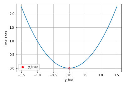
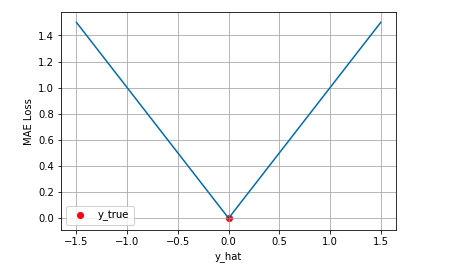
由于训练结构参数 θ 时,网络的权重是冻结的,我们希望该约束项的值在训练的早期阶段就尽快下降到0,并长时间保持在0(在0附近梯度很大),这样可以有较长的时间可以来训练结构参数 θ,但MAE/MSE不满足这个要求,因为在0附近MSE的梯度为0,MAE的梯度恒定。
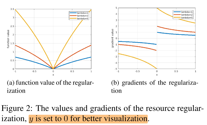
因此实际采用的正则项的形式为: \(\mathcal{R}_{\log }(x, y)=\log (|x-y|+1) \qquad (10)\)
\(R_{log}\) 在x=y处不可导,可以使用次梯度(sub-gradient)来替代
如图2,取y=0,x越靠近0,\(R_{log}\) 的梯度越大:
结构参数θ 对称的权重衰减(Symmetric Weight Decay)
&& To further expand search space, we propose a symmetric weight decay on the weights of gates, which is inspired by the subgradient of the regularization loss:
为了进一步扩大搜索空间,我们提出了对门的权重进行对称的权重衰减,其灵感来自于正则化损失的次梯度:
\(\frac{\partial \mathcal{R}_{\mathrm{log}}}{\partial \theta_{l, c}}=\left\{\begin{array}{ll}\eta_{l} \cdot \frac{1}{|\hat{T}-p T|+1} \cdot \frac{\hat{T}-p T}{|\hat{T}-p T|}, & \text { if } \hat{T} \neq p T \\ 0, & \text { if } \hat{T}=p T\end{array}\right. \qquad (11)\)
其中 \(\eta_{l}=k_{l}^{2} \cdot \frac{\mathbf{1}^{T} \mathbf{g}_{l-1}}{\mathcal{G}_{l}} \cdot w_{l} \cdot h_{l}\)
\((\widehat{\mathrm{FLOPs}})_{l}=k_{l} \cdot k_{l} \cdot \frac{\mathbf{1}^{T} \mathbf{g}_{l-1}}{\mathcal{G}_{l}} \cdot \mathbf{1}^{T} \mathbf{g}_{l} \cdot w_{l} \cdot h_{l} \qquad (8)\)
\(R_{log}\) 就像对 θ 进行权重衰减一样
&& Based on above arguments, we can explore larger search spaces by applying symmetric weight decay on each \(θ_{l,c}\) .
The goal of doing this is to slow down the pace of gate parameters to become deterministic (approach 0 or 1).
As a result, the search space is enlarged:
\(\theta_{l, c}=\theta_{l, c}-\beta \operatorname{sign}\left(\theta_{l, c}-0.5\right) \qquad (12)\)
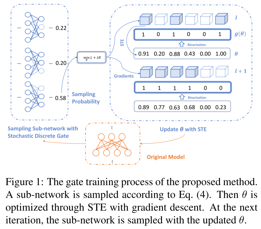
DMC Algorithm
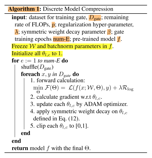
&& 左边是前向,右边是反向
前向:以 \(\Theta\) 的概率采样一个子网,做前向
反向:计算loss,用STE更新 \(\Theta\)
Experiments
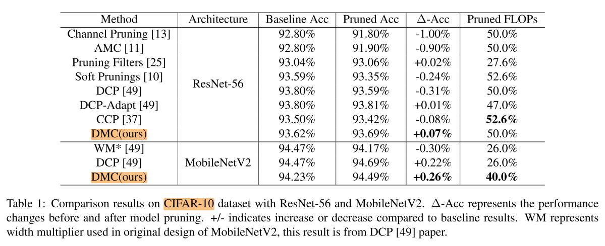
CIFAR-10
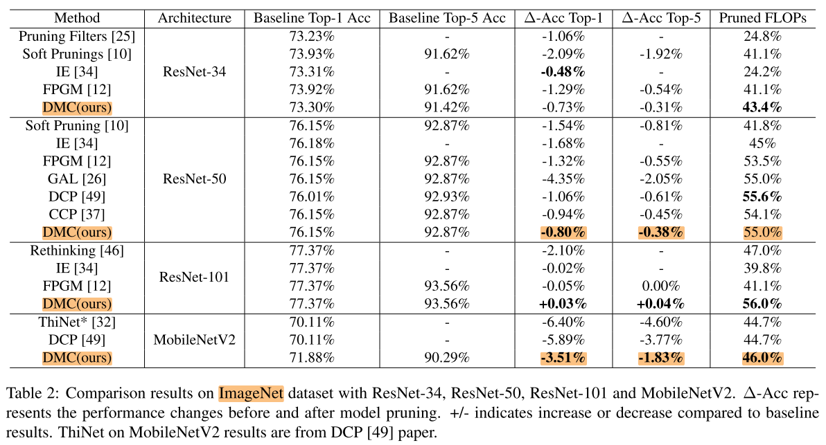
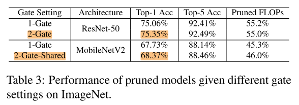
ImageNet
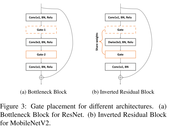
Impact of Gate Placement
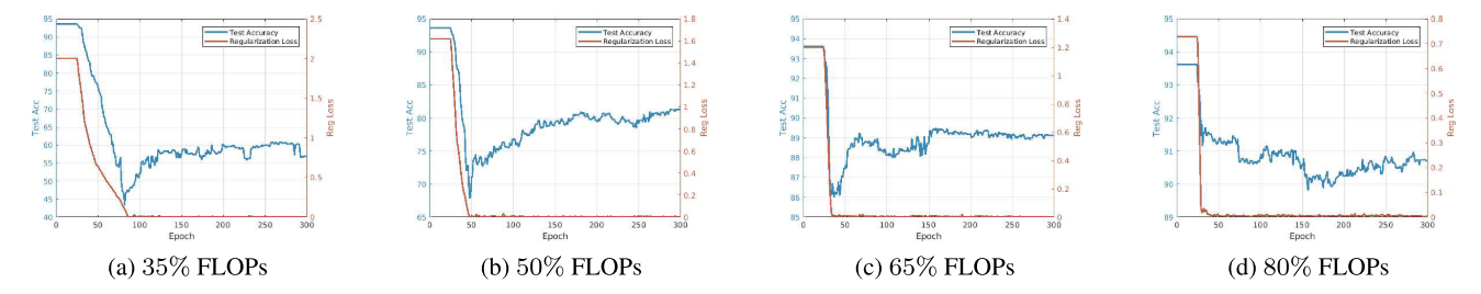
Understanding the Training of Discrete Gates
test-acc VS Regularization Loss
Regularization Loss先急剧下降,然后保持在0附近
同时test-acc也是先急剧下降,再缓慢上升
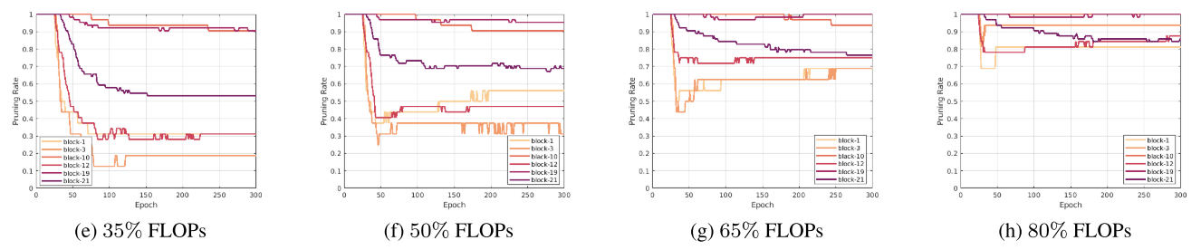
不同层的剪枝率变化情况
有些层的剪枝率一开始逐渐下降,后面会逐渐恢复,说明这些层有的通道被逐渐恢复了(recall)
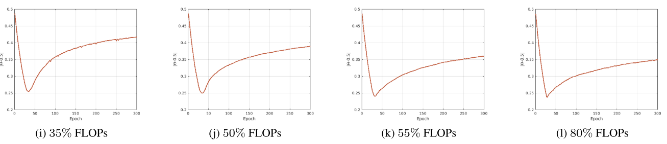
S值的变化
\(\mathcal{S}=\frac{\sum_{l=1}^{L} \sum_{c=1}^{C_{l}}\left|\theta_{l, c}-0.5\right|}{n}\)
s越小,说明θ趋于随机分布
s越接近0,说明θ趋于0,1两极分布

 浙公网安备 33010602011771号