day 10 逻辑回归实例代码
代码加注释
import numpy as np
import tensorflow.compat.v1 as tf
import matplotlib.pyplot as plt
from tensorflow.examples.tutorials.mnist import input_data
tf.compat.v1.disable_eager_execution()
tf.disable_v2_behavior()
#加载mnist数据集
mnist = input_data.read_data_sets("C:/Users/chenqi/Desktop/data/mnist", one_hot=True)
trainimg = mnist.train.images
trainlabel = mnist.train.labels
testimg = mnist.test.images
testlabel = mnist.test.labels
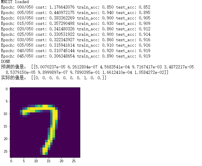
print ("MNIST loaded")
#构造计算图,使用占位符函数构造二维浮点数变量x,y
x = tf.placeholder("float", [None, 784])
y = tf.placeholder("float", [None, 10]) # None is for infinite
#初始化二维参数变量W,b
W = tf.Variable(tf.zeros([784, 10]))
b = tf.Variable(tf.zeros([10]))
#构造逻辑回归模型
#通过softmax将线性结果分类处理
#返回一个10维矩阵,[None,784]*[784,10]=[None,10]
actv = tf.nn.softmax(tf.matmul(x, W) + b)
#构造代价函数(交叉熵损失函数)
#-y*tf.log(pred):交叉熵代价函数
#reduce_sum() 求和
#reduce_mean() 求平均值,返回数字
cost = tf.reduce_mean(-tf.reduce_sum(y*tf.log(actv), reduction_indices=1))
#学习率
learning_rate = 0.01
#定义梯度下降优化器(使用梯度下降法求最小值,即最优解)
optm = tf.train.GradientDescentOptimizer(learning_rate).minimize(cost)
#argmax返回数组中最大元素的位置 0代表按列算,1代表按行算
#tf.equal() 返回布尔值,判断对应元素是否相等,相等返回1,否则返回0
#tf.cast()将布尔值转换为浮点数
pred = tf.equal(tf.argmax(actv, 1), tf.argmax(y, 1))
#样本集准确率
accr = tf.reduce_mean(tf.cast(pred, "float"))
# 初始化全部变量
init = tf.global_variables_initializer()
#训练整个样本集次数
training_epochs = 50
#定义批量梯度下降次数,每100张图计算一次
batch_size = 100
#每训练整个样本集五次打印一下结果
display_step = 5
#使用tf.Session()创建Session会话对象,会话封装了Tensorflow运行时的状态和控制。
sess = tf.Session()
sess.run(init)
#for循环跑50次整个训练集
for epoch in range(training_epochs):
#记录每次训练集的误差
avg_cost = 0.
#一次训练一百个,总数55000,训练550次把全部样本集训练完
num_batch = int(mnist.train.num_examples/batch_size)
for i in range(num_batch):
batch_xs, batch_ys = mnist.train.next_batch(batch_size)
#训练模型
sess.run(optm, feed_dict={x: batch_xs, y: batch_ys})
feeds = {x: batch_xs, y: batch_ys}
avg_cost += sess.run(cost, feed_dict=feeds)/num_batch
#每五次打印结果
if epoch % display_step == 0:
feeds_train = {x: batch_xs, y: batch_ys}
feeds_test = {x: mnist.test.images, y: mnist.test.labels}
train_acc = sess.run(accr, feed_dict=feeds_train)
test_acc = sess.run(accr, feed_dict=feeds_test)
print ("Epoch: %03d/%03d cost: %.9f train_acc: %.3f test_acc: %.3f"
% (epoch, training_epochs, avg_cost, train_acc, test_acc))
print ("DONE")
print('预测的值是:',sess.run(actv, feed_dict={x: np.array([mnist.test.images[254]]), y: np.array([mnist.test.labels[254]])}))
print('实际的值是:',sess.run(y, feed_dict={x: np.array([mnist.test.images[254]]), y: np.array([mnist.test.labels[254]])}))
one_pic_arr = np.reshape(mnist.test.images[254], (28, 28))
pic_matrix = np.matrix(one_pic_arr, dtype="float")
plt.imshow(pic_matrix)
plt.show()
运行截图
逻辑回归
-
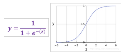
逻辑回归通过Sigmoid函数保证输出的值在[0,1]之间,该函数可以将全体实数映射到[0,1],从而将线性的输出转换为[0,1]的数。其定义与图像如下
-
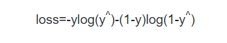
前面我们讲过,在逻辑回归中如果采用均方差的损失函数,带入sigmoid会得到一个非凸函数,这类函数会有多个极小值,采用梯度下降法便无法求得最优解。因此在逻辑回归中采用对数损失函数
-
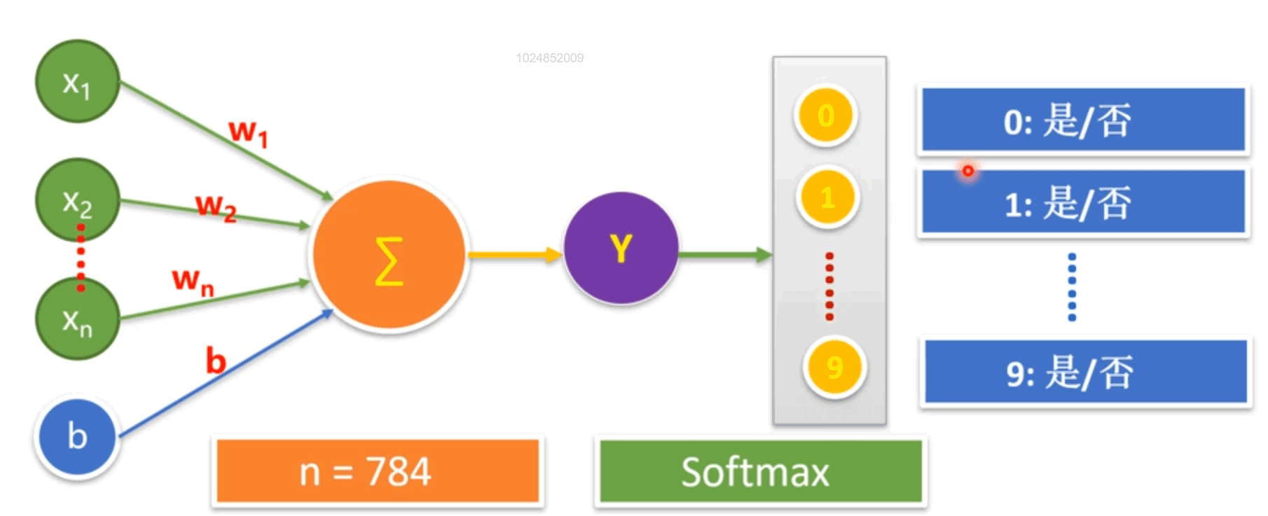
在手写数字识别中,通过单层神经元产生连续的输出值y,将y再输入到softmax层处理,经过函数计算将结果映射为0~9每个数字对应的概率,概率越大表示该图片越像某个数字,所有数字的概率之和为1
-
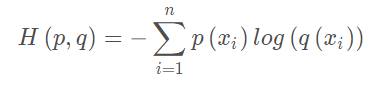
交叉熵损失函数:交叉熵用于刻画两个概率分布之间的距离,其中p代表正确答案,q代表预测值,交叉熵越小距离越近,从而模型的预测越准确。例如正确答案为(1,0,0),甲模型预测为(0.5,0.2,0.3),其交叉熵=-1log0.5≈0.3,乙模型(0.7,0.1,0.2),其交叉熵=-1log0.7≈0.15,所以乙模型预测更准确
-
x(图片特征值):x=tf.placeholder(tf.float32,[None,784]) 此代码将图片表示为若干行,784列的数组,这个None就是为了向量化,可以一次训练多个图片。
w(特征值对应的权重):一开始这个值是随即设置,随着我们的不断训练得到最佳的权重
y(正确的结果):此结果来自MNIST标签训练集,此数据用于与我们机器学习预测的结果相比较,看是否预测正确,同时计算准确率
accr:机器学习预测的结果。
training_epochs:指的是遍历全部样本集的次数
batch_size:我们需要分好几次来遍历完全样本集,batch_size指的是每次分步提取出数据集的数量,例如样本集有5000个,batch_size=100时代表每次需分析100张图片,共迭代50次全部完成。向量化的体现,一次一个效率太低通过向量化实现每次100张图片。

 浙公网安备 33010602011771号