tensorflow2.0的学习

接上一篇：

https://www.cnblogs.com/charlesblc/p/15978168.html

 

今天主要看这个教材：

https://tensorflow.google.cn/tutorials?hl=zh-cn

 

图像分类

# TensorFlow and tf.keras
import tensorflow as tf
from tensorflow import keras

# Helper libraries
import numpy as np
import matplotlib.pyplot as plt

print(tf.__version__)

2.3.0

 

 

本指南使用 Fashion MNIST 数据集，该数据集包含 10 个类别的 70,000 个灰度图像。这些图像以低分辨率（28x28 像素）展示了单件衣物

 

fashion_mnist = keras.datasets.fashion_mnist

(train_images, train_labels), (test_images, test_labels) = fashion_mnist.load_data()

标签    类
0    T恤/上衣
1    裤子
2    套头衫
3    连衣裙
4    外套
5    凉鞋
6    衬衫
7    运动鞋
8    包
9    短靴

 

 

 

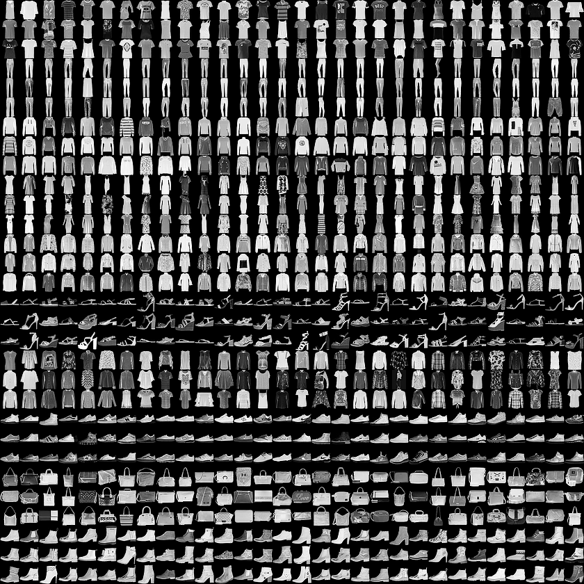
class_names = ['T-shirt/top', 'Trouser', 'Pullover', 'Dress', 'Coat',
               'Sandal', 'Shirt', 'Sneaker', 'Bag', 'Ankle boot']

train_images.shape

(60000, 28, 28)

len(train_labels)

60000

train_labels

array([9, 0, 0, ..., 3, 0, 5], dtype=uint8)

plt.figure()
plt.imshow(train_images[0])
plt.colorbar()
plt.grid(False)
plt.show()

train_images = train_images / 255.0

test_images = test_images / 255.0

plt.figure(figsize=(10,10))
for i in range(25):
    plt.subplot(5,5,i+1)
    plt.xticks([])
    plt.yticks([])
    plt.grid(False)
    plt.imshow(train_images[i], cmap=plt.cm.binary)
    plt.xlabel(class_names[train_labels[i]])
plt.show()

 

 

 

 

model = keras.Sequential([
    keras.layers.Flatten(input_shape=(28, 28)),
    keras.layers.Dense(128, activation='relu'),
    keras.layers.Dense(10)
])

该网络的第一层 tf.keras.layers.Flatten 将图像格式从二维数组（28 x 28 像素）转换成一维数组（28 x 28 = 784 像素）。将该层视为图像中未堆叠的像素行并将其排列起来。该层没有要学习的参数，它只会重新格式化数据。

展平像素后，网络会包括两个 tf.keras.layers.Dense 层的序列。它们是密集连接或全连接神经层。第一个 Dense 层有 128 个节点（或神经元）。第二个（也是最后一个）层会返回一个长度为 10 的 logits 数组。每个节点都包含一个得分，用来表示当前图像属于 10 个类中的哪一类。

 

编译模型

在准备对模型进行训练之前，还需要再对其进行一些设置。以下内容是在模型的编译步骤中添加的：

• 损失函数 - 用于测量模型在训练期间的准确率。您会希望最小化此函数，以便将模型“引导”到正确的方向上。
• 优化器 - 决定模型如何根据其看到的数据和自身的损失函数进行更新。
• 指标 - 用于监控训练和测试步骤。以下示例使用了准确率，即被正确分类的图像的比率。

 

model.compile(optimizer='adam',
              loss=tf.keras.losses.SparseCategoricalCrossentropy(from_logits=True),
              metrics=['accuracy'])

model.fit(train_images, train_labels, epochs=10)

test_loss, test_acc = model.evaluate(test_images,  test_labels, verbose=2)

print('\nTest accuracy:', test_acc)

313/313 - 0s - loss: 0.3726 - accuracy: 0.8635

Test accuracy: 0.8634999990463257

 

训练准确率和测试准确率之间的差距代表过拟合。

 

过拟合的模型会“记住”训练数据集中的噪声和细节，从而对模型在新数据上的表现产生负面影响。

 

在模型经过训练后，您可以使用它对一些图像进行预测。模型具有线性输出，即 logits。您可以附加一个 softmax 层，将 logits 转换成更容易理解的概率。

 

probability_model = tf.keras.Sequential([model, 
                                         tf.keras.layers.Softmax()])

predictions = probability_model.predict(test_images)

predictions[0]

array([6.9982241e-07, 5.5403369e-08, 1.8353174e-07, 1.4761626e-07,
       2.4380807e-07, 1.9273469e-04, 1.8122660e-06, 6.5027133e-02,
       1.7891599e-06, 9.3477517e-01], dtype=float32)

np.argmax(predictions[0])

9

画图

def plot_image(i, predictions_array, true_label, img):
  predictions_array, true_label, img = predictions_array, true_label[i], img[i]
  plt.grid(False)
  plt.xticks([])
  plt.yticks([])

  plt.imshow(img, cmap=plt.cm.binary)

  predicted_label = np.argmax(predictions_array)
  if predicted_label == true_label:
    color = 'blue'
  else:
    color = 'red'

  plt.xlabel("{} {:2.0f}% ({})".format(class_names[predicted_label],
                                100*np.max(predictions_array),
                                class_names[true_label]),
                                color=color)

def plot_value_array(i, predictions_array, true_label):
  predictions_array, true_label = predictions_array, true_label[i]
  plt.grid(False)
  plt.xticks(range(10))
  plt.yticks([])
  thisplot = plt.bar(range(10), predictions_array, color="#777777")
  plt.ylim([0, 1])
  predicted_label = np.argmax(predictions_array)

  thisplot[predicted_label].set_color('red')
  thisplot[true_label].set_color('blue')


i = 0
plt.figure(figsize=(6,3))
plt.subplot(1,2,1)
plot_image(i, predictions[i], test_labels, test_images)
plt.subplot(1,2,2)
plot_value_array(i, predictions[i],  test_labels)
plt.show()


# Plot the first X test images, their predicted labels, and the true labels.
# Color correct predictions in blue and incorrect predictions in red.
num_rows = 5
num_cols = 3
num_images = num_rows*num_cols
plt.figure(figsize=(2*2*num_cols, 2*num_rows))
for i in range(num_images):
  plt.subplot(num_rows, 2*num_cols, 2*i+1)
  plot_image(i, predictions[i], test_labels, test_images)
  plt.subplot(num_rows, 2*num_cols, 2*i+2)
  plot_value_array(i, predictions[i], test_labels)
plt.tight_layout()
plt.show()

 

文本分类预测

imdb = keras.datasets.imdb

(train_data, train_labels), (test_data, test_labels) = imdb.load_data(num_words=10000)

Downloading data from https://storage.googleapis.com/tensorflow/tf-keras-datasets/imdb.npz
17465344/17464789 [==============================] - 0s 0us/step

反向查找单词

# 一个映射单词到整数索引的词典
word_index = imdb.get_word_index()

# 保留第一个索引
word_index = {k:(v+3) for k,v in word_index.items()}
word_index["<PAD>"] = 0
word_index["<START>"] = 1
word_index["<UNK>"] = 2  # unknown
word_index["<UNUSED>"] = 3

reverse_word_index = dict([(value, key) for (key, value) in word_index.items()])

def decode_review(text):
    return ' '.join([reverse_word_index.get(i, '?') for i in text])

填充长度

train_data = keras.preprocessing.sequence.pad_sequences(train_data,
                                                        value=word_index["<PAD>"],
                                                        padding='post',
                                                        maxlen=256)

test_data = keras.preprocessing.sequence.pad_sequences(test_data,
                                                       value=word_index["<PAD>"],
                                                       padding='post',
                                                       maxlen=256)

模型结构

# 输入形状是用于电影评论的词汇数目（10,000 词）
vocab_size = 10000

model = keras.Sequential()
model.add(keras.layers.Embedding(vocab_size, 16))
model.add(keras.layers.GlobalAveragePooling1D())
model.add(keras.layers.Dense(16, activation='relu'))
model.add(keras.layers.Dense(1, activation='sigmoid'))

model.summary()

Model: "sequential"
_________________________________________________________________
Layer (type)                 Output Shape              Param #   
=================================================================
embedding (Embedding)        (None, None, 16)          160000    
_________________________________________________________________
global_average_pooling1d (Gl (None, 16)                0         
_________________________________________________________________
dense (Dense)                (None, 16)                272       
_________________________________________________________________
dense_1 (Dense)              (None, 1)                 17        
=================================================================
Total params: 160,289
Trainable params: 160,289
Non-trainable params: 0
_________________________________________________________________

1. 第一层是嵌入（Embedding）层。该层采用整数编码的词汇表，并查找每个词索引的嵌入向量（embedding vector）。这些向量是通过模型训练学习到的。向量向输出数组增加了一个维度。得到的维度为：(batch, sequence, embedding)。
2. 接下来，GlobalAveragePooling1D 将通过对序列维度求平均值来为每个样本返回一个定长输出向量。这允许模型以尽可能最简单的方式处理变长输入。
3. 该定长输出向量通过一个有 16 个隐层单元的全连接（Dense）层传输。
4. 最后一层与单个输出结点密集连接。使用 Sigmoid 激活函数，其函数值为介于 0 与 1 之间的浮点数，表示概率或置信度。

 

您可以选择 mean_squared_error 。但是，一般来说 binary_crossentropy 更适合处理概率——它能够度量概率分布之间的“距离”，或者在我们的示例中，指的是度量 ground-truth 分布与预测值之间的“距离”。

稍后，当我们研究回归问题（例如，预测房价）时，我们将介绍如何使用另一种叫做均方误差的损失函数。

 

model.compile(optimizer='adam',
              loss='binary_crossentropy',
              metrics=['accuracy'])

看下这里的损失函数，和图像算法里面是不一样的。因为图像算法的输出是一个数组，需要进一步操作。而这里的输出是一个sigmoid计算之后的结果。

 

在训练时，我们想要检查模型在未见过的数据上的准确率（accuracy）。通过从原始训练数据中分离 10,000 个样本来创建一个验证集。（为什么现在不使用测试集？我们的目标是只使用训练数据来开发和调整模型，然后只使用一次测试数据来评估准确率（accuracy））。

x_val = train_data[:10000]
partial_x_train = train_data[10000:]

y_val = train_labels[:10000]
partial_y_train = train_labels[10000:]

 

history = model.fit(partial_x_train,
                    partial_y_train,
                    epochs=40,
                    batch_size=512,
                    validation_data=(x_val, y_val),
                    verbose=1)

results = model.evaluate(test_data,  test_labels, verbose=2)

print(results)

782/782 - 1s - loss: 0.3298 - accuracy: 0.8729
[0.32977813482284546, 0.8728799819946289]

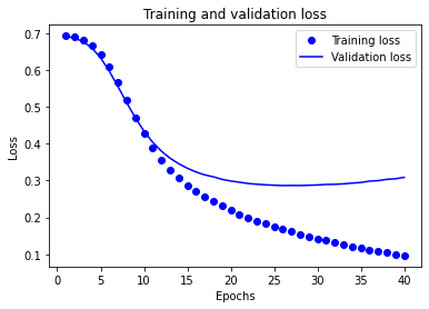
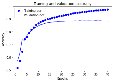
创建一个准确率（accuracy）和损失值（loss）随时间变化的图表

model.fit() 返回一个 History 对象，该对象包含一个字典，其中包含训练阶段所发生的一切事件：

history_dict = history.history
history_dict.keys()

dict_keys(['loss', 'accuracy', 'val_loss', 'val_accuracy'])


import matplotlib.pyplot as plt

acc = history_dict['accuracy']
val_acc = history_dict['val_accuracy']
loss = history_dict['loss']
val_loss = history_dict['val_loss']

epochs = range(1, len(acc) + 1)

# “bo”代表 "蓝点"
plt.plot(epochs, loss, 'bo', label='Training loss')
# b代表“蓝色实线”
plt.plot(epochs, val_loss, 'b', label='Validation loss')
plt.title('Training and validation loss')
plt.xlabel('Epochs')
plt.ylabel('Loss')
plt.legend()

plt.show()

plt.clf()   # 清除数字

plt.plot(epochs, acc, 'bo', label='Training acc')
plt.plot(epochs, val_acc, 'b', label='Validation acc')
plt.title('Training and validation accuracy')
plt.xlabel('Epochs')
plt.ylabel('Accuracy')
plt.legend()

plt.show()

 

 

我们将使用包含 Internet Movie Database 中的 50,000 条电影评论文本的 IMDB 数据集。先将这些评论分为两组，其中 25,000 条用于训练，另外 25,000 条用于测试。训练组和测试组是均衡的，也就是说其中包含相等数量的正面评价和负面评价。

 

这里面能提高效果的就是利用预训练的嵌入向量。

https://tensorflow.google.cn/tutorials/keras/text_classification_with_hub?hl=zh-cn

 

一个模型需要一个损失函数和一个优化器来训练。由于这是一个二元分类问题，并且模型输出 logit（具有线性激活的单一单元层），因此，我们将使用 binary_crossentropy 损失函数。 

 

本 notebook 使用经典的 Auto MPG 数据集，构建了一个用来预测70年代末到80年代初汽车燃油效率的模型。为了做到这一点，我们将为该模型提供许多那个时期的汽车描述。这个描述包含：气缸数，排量，马力以及重量。

 

import pathlib

import matplotlib.pyplot as plt
import pandas as pd
import seaborn as sns

import tensorflow as tf

from tensorflow import keras
from tensorflow.keras import layers

print(tf.__version__)

 

"Origin" 列实际上代表分类，而不仅仅是一个数字。所以把它转换为独热码 （one-hot）。

感觉这个操作对于效果是有一定帮助的。

 

使用 .summary 方法来打印该模型的简单描述。

 

model.summary()

Model: "sequential"
_________________________________________________________________
Layer (type)                 Output Shape              Param #   
=================================================================
dense (Dense)                (None, 64)                640       
_________________________________________________________________
dense_1 (Dense)              (None, 64)                4160      
_________________________________________________________________
dense_2 (Dense)              (None, 1)                 65        
=================================================================
Total params: 4,865
Trainable params: 4,865
Non-trainable params: 0
_________________________________________________________________

 

我们将使用一个 EarlyStopping callback 来测试每个 epoch 的训练条件。如果经过一定数量的 epochs 后没有改进，则自动停止训练。

model = build_model()

# patience 值用来检查改进 epochs 的数量
early_stop = keras.callbacks.EarlyStopping(monitor='val_loss', patience=10)

history = model.fit(normed_train_data, train_labels, epochs=EPOCHS,
                    validation_split = 0.2, verbose=0, callbacks=[early_stop, PrintDot()])

plot_history(history)

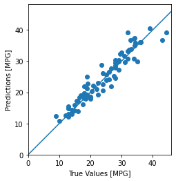
使用测试集中的数据预测：

test_predictions = model.predict(normed_test_data).flatten()

plt.scatter(test_labels, test_predictions)
plt.xlabel('True Values [MPG]')
plt.ylabel('Predictions [MPG]')
plt.axis('equal')
plt.axis('square')
plt.xlim([0,plt.xlim()[1]])
plt.ylim([0,plt.ylim()[1]])
_ = plt.plot([-100, 100], [-100, 100])

 

结论

本笔记本 (notebook) 介绍了一些处理回归问题的技术。

• 均方误差（MSE）是用于回归问题的常见损失函数（分类问题中使用不同的损失函数）。
• 类似的，用于回归的评估指标与分类不同。 常见的回归指标是平均绝对误差（MAE）。
• 当数字输入数据特征的值存在不同范围时，每个特征应独立缩放到相同范围。
• 如果训练数据不多，一种方法是选择隐藏层较少的小网络，以避免过度拟合。
• 早期停止是一种防止过度拟合的有效技术。

 

 

 

在训练期间保存模型（以 checkpoints 形式保存）

您可以使用经过训练的模型而无需重新训练，或者在训练过程中断的情况下从离开处继续训练。tf.keras.callbacks.ModelCheckpoint 回调允许您在训练期间和结束时持续保存模型。

 

checkpoint_path = "training_1/cp.ckpt"
checkpoint_dir = os.path.dirname(checkpoint_path)

# Create a callback that saves the model's weights
cp_callback = tf.keras.callbacks.ModelCheckpoint(filepath=checkpoint_path,
                                                 save_weights_only=True,
                                                 verbose=1)

# Train the model with the new callback
model.fit(train_images, 
          train_labels,  
          epochs=10,
          validation_data=(test_images, test_labels),
          callbacks=[cp_callback])  # Pass callback to training

# This may generate warnings related to saving the state of the optimizer.
# These warnings (and similar warnings throughout this notebook)
# are in place to discourage outdated usage, and can be ignored.

加载和复用模型

# Create a basic model instance
model = create_model()

# Evaluate the model
loss, acc = model.evaluate(test_images, test_labels, verbose=2)
print("Untrained model, accuracy: {:5.2f}%".format(100 * acc))


32/32 - 0s - loss: 2.3609 - sparse_categorical_accuracy: 0.1150
Untrained model, accuracy: 11.50%


# Loads the weights
model.load_weights(checkpoint_path)

# Re-evaluate the model
loss, acc = model.evaluate(test_images, test_labels, verbose=2)
print("Restored model, accuracy: {:5.2f}%".format(100 * acc))


32/32 - 0s - loss: 0.4329 - sparse_categorical_accuracy: 0.8640
Restored model, accuracy: 86.40%

 

Checkpoints 包含：

• 一个或多个包含模型权重的分片。
• 一个索引文件，指示哪些权重存储在哪个分片中。

如果您在一台计算机上训练模型，您将获得一个具有如下后缀的分片：.data-00000-of-00001

 

手动保存权重

使用 Model.save_weights 方法手动保存权重。

 

保存整个模型

调用 model.save 将保存模型的结构，权重和训练配置保存在单个文件/文件夹中。这可以让您导出模型，以便在不访问原始 Python 代码*的情况下使用它。因为优化器状态（optimizer-state）已经恢复，您可以从中断的位置恢复训练。

 

整个模型可以保存为两种不同的文件格式（SavedModel 和 HDF5）。TensorFlow SavedModel 格式是 TF2.x 中的默认文件格式。但是，模型能够以 HDF5 格式保存。下面详细介绍了如何以两种文件格式保存整个模型。

 

HDF5 和 SavedModel 之间的主要区别在于，HDF5 使用对象配置来保存模型架构，而 SavedModel 则保存执行计算图。因此，SavedModel 能够在不需要原始代码的情况下保存自定义对象，如子类模型和自定义层。