scorecardpy 介绍

前语：平时计算变量IV值时也有调用过scorecardpy库，不过总体来说使用次数不多，对此功能也不是很熟悉，一般都是使用自己内部的库，但是涉及到去其他公司建模，或者是一个封闭的环境时，常常不能使用自己的东西，这就得使用toad或者scorecardpy，下面简单介绍一下，不过着重点还是一下三点：

（1）将iv(输出是一个字典）输出结果，转化成pd.df；iv参数的使用；

（2）转换评分卡 ，scorecardpy内置的模型时sklearn 的逻辑回归，如果使用其他的，比如statsmodels.api 的逻辑回归，又该如何应对；

（3）如果使用scorecardpy，整个建模流程是如何。

下面开始本次学习之旅，以及解决上面三个问题。

 

一、导入数据

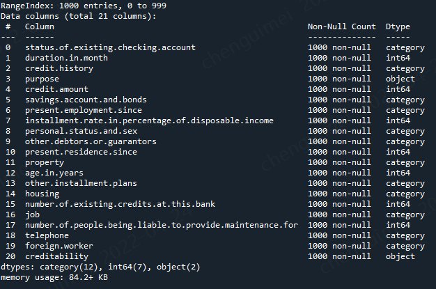
使用的是scorecardpy内置的数据作为例子

import scorecardpy as sc

# 加载德国信用卡相关数据集
dat = sc.germancredit()
dat.info()

 

二、计算变量iv

看其他的介绍文档里面，这一步是变量刷选，但是我觉得首先要对变量的整体情况有一定了解，再去刷选变量，所以这一步先计算变量iv 

使用函数是sc.woebin()

sc.woebin??

def woebin(dt, y, x=None, 
           var_skip=None, breaks_list=None, special_values=None, 
           stop_limit=0.1, count_distr_limit=0.05, bin_num_limit=8, 
           # min_perc_fine_bin=0.02, min_perc_coarse_bin=0.05, max_num_bin=8, 
           positive="bad|1", no_cores=None, print_step=0, method="tree",
           ignore_const_cols=True, ignore_datetime_cols=True, 
           check_cate_num=True, replace_blank=True, 
           save_breaks_list=None, **kwargs):

woebin()可针对数值型和类别型变量生成最优分箱结果，方法可选择决策树分箱、卡方分箱或自定义分箱。其他各参数的含义如下：

• var_skip: 设置需要跳过分箱操作的变量；
• breaks_list: 切分点列表，默认为空。如果非空，则按设置的切分点进行分箱处理；
• special_values: 设置需要单独分箱的值，默认为空；
• count_distr_limit: 设置分箱占比的最小值，一般可接受范围为0.01-0.2，默认值为0.05；
• stop_limit: 当IV值的增长率小于所设置的stop_limit，或卡方值小于qchisq(1-stoplimit, 1)时，停止分箱。一般可接受范围为0-0.5，默认值为0.1；
• bin_num_limit: 该参数为整数，代表最大分箱数。
• positive: 指定样本中正样本对应的标签，默认为"bad|1"；
• no_cores: 设置用于并行计算的 CPU 数目；
• print_step: 该参数为非负数，默认值为1。若print_step>0，每次迭代会输出变量名。若iteration=0或no_cores>1，不会输出任何信息；
• method: 设置分箱方法，可设置"tree"（决策树）或"chimerge"（卡方），默认值为"tree";
• ignore_const_cols: 是否忽略常数列，默认值为True，即忽略常数列；
• ignore_datetime_cols: 是否忽略日期列，默认值为True，即忽略日期列；
• check_cate_num: 检查类别变量中枚举值数目是否大于50，默认值为True，即自动进行检查。若枚举值过多，会影响分箱过程的速度；
• replace_blank: 设置是否将空值填为None，默认为True。

一般设置这三个参数即可，其余的使用默认参数

#如果special_values=-1000，可以这样表示，就会将-1000作为单独的一箱
bins = sc.woebin(dat, y="creditability",count_distr_limit=0.05, bin_num_limit=5)

 

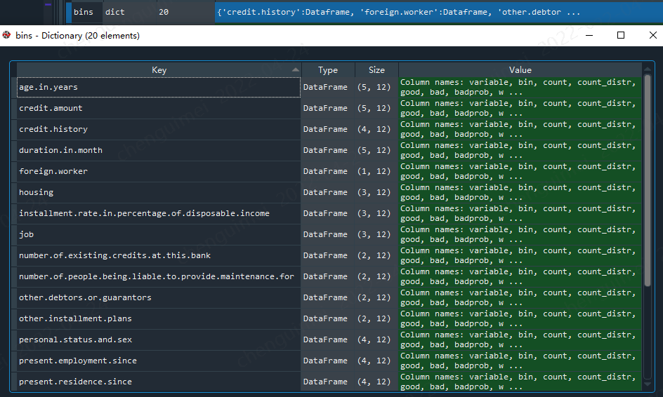
 我们需要将dict转为pd.df 

import pandas as pd
iv_data = pd.DataFrame()
for i in dat.columns[0:-1]:
    iv_data = iv_data.append(bins[i])

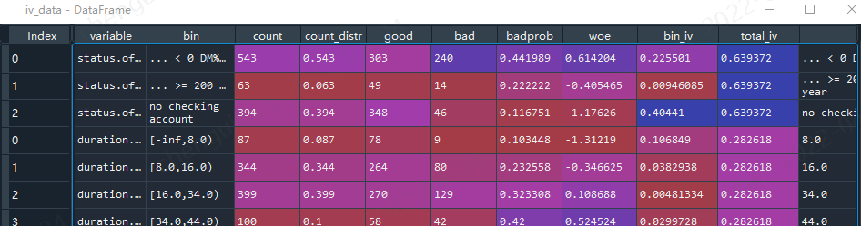
 这样就比较好看。且容易分析比较

当然你也可以使用画图的形式（但是图片占用内存过大，且当变量特别多时候，看起来也很困难，因此我一般不使用），就会输出每个变量的分箱图片。

sc.woebin_plot(bins)

 

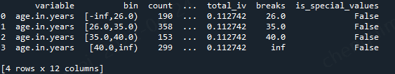
调箱可以这样处理，breaks_list，参数是dict形式

breaks_adj = {
    'age.in.years': [26, 35, 40],
    'other.debtors.or.guarantors': ["none", "co-applicant%,%guarantor"]
}
bins_adj = sc.woebin(dat, y="creditability", breaks_list=breaks_adj)
bins_adj['age.in.years']

 

三、划分数据集

sc内置了一个划分数据集的函数，但其实是使用df.sample()函数，里面也2个参数，可以自己设置

train, test = sc.split_df(dat, 'creditability').values()

#def split_df(dt, y=None, ratio=0.7, seed=186)

 

四、刷选变量

先介绍sc里面的用法，var_filter根据IV 值小于0.02，或缺失率大于95%，或同值率（除空值外）大于95% 去剔除变量

def var_filter(dt, y, x=None, iv_limit=0.02, missing_limit=0.95,  
               identical_limit=0.95, var_rm=None, var_kp=None, 
               return_rm_reason=False, positive='bad|1')

其中各参数含义如下：

• varrm可设置强制保留的变量，默认为空；
• varkp可设置强制剔除的变量，默认为空；
• return_rm_reason可设置是否返回剔除原因，默认为不返回（False）；
• positive可设置坏样本对应的值，默认为“bad|1”。

dt_s = sc.var_filter(dat, y="creditability")

其实更建议手动挑选，因为做评分卡需要模型有可解释性，也就是要求模型入模变量符合业务解释，要求单调性等等，单纯的iv可能选择不了最符合的。

不过变量很多时，可以用来做初刷。

 

五、woe转换

使用woebin_ply()函数对变量进行woe变换，最后变量是以woe结尾

cols = list(dt_s.columns)
train_woe = sc.woebin_ply(train[cols], bins_adj)
test_woe = sc.woebin_ply(test[cols], bins_adj)

train_woe.columns
'''
Index(['creditability', 'credit.history_woe', 'purpose_woe',
       'other.debtors.or.guarantors_woe', 'duration.in.month_woe',
       'present.employment.since_woe', 'savings.account.and.bonds_woe',
       'installment.rate.in.percentage.of.disposable.income_woe',
       'status.of.existing.checking.account_woe', 'age.in.years_woe',
       'housing_woe', 'other.installment.plans_woe', 'credit.amount_woe',
       'property_woe'],
      dtype='object')
'''

 

六、模型训练

需要注意，lr.coef_，lr.intercept_ ，转换成评分卡时候能够用得到。

y_train = train_woe.loc[:,'creditability']
X_train = train_woe.loc[:,train_woe.columns != 'creditability']
y_test = test_woe.loc[:,'creditability']
X_test = test_woe.loc[:,train_woe.columns != 'creditability']

# 逻辑回归 ------
from sklearn.linear_model import LogisticRegression
lr = LogisticRegression(penalty='l1', C=0.9, solver='saga', n_jobs=-1)
lr.fit(X_train, y_train)
lr.coef_
lr.intercept_

# 预测
train_pred = lr.predict_proba(X_train)[:,1]
test_pred = lr.predict_proba(X_test)[:,1]

有一个系数为0，说明该系数对应的变量是没有用处的。

 

当然我们也可以使用statsmodels.api 的逻辑回归

import pandas as pd
import matplotlib.pyplot as plt #导入图像库
import matplotlib
import seaborn as sns
import statsmodels.api as sm
from sklearn.metrics import roc_curve, auc
from sklearn.model_selection import train_test_split

target_train = y_train.map({'good':0,'bad':1})
target_test = y_test.map({'good':0,'bad':1})

X1=sm.add_constant(X_train)   #在X前加上一列常数1，方便做带截距项的回归
logit=sm.Logit(target_train.values,X1.astype(float))
result=logit.fit()
result.summary()
result.params

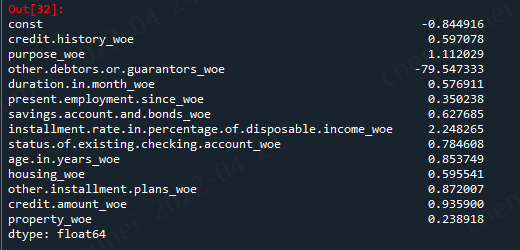
 但是有一个变量的系数是负值，意味着这些变量之间存在着共线性，我们需要将次去掉

model_cols = ['credit.history_woe', 'purpose_woe', #'other.debtors.or.guarantors_woe',
       'duration.in.month_woe', 'present.employment.since_woe',
       'savings.account.and.bonds_woe',
       'installment.rate.in.percentage.of.disposable.income_woe',
       'status.of.existing.checking.account_woe', 'age.in.years_woe',
       'housing_woe', 'other.installment.plans_woe', 'credit.amount_woe',
       'property_woe']

X1=sm.add_constant(X_train[model_cols])   #在X前加上一列常数1，方便做带截距项的回归
logit=sm.Logit(target_train.values,X1.astype(float))
result=logit.fit()
result.summary()
result.params

 这样子就OK了

#预测
#训练集
resu_01 = result.predict(X1)

#测试集
X2 = sm.add_constant(X_test)
resu_02 = result.predict(X2.astype(float))

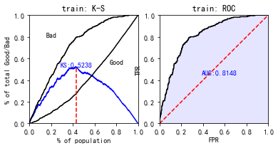
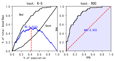
查看模型效果

#构建一个画auc和ks的图像
from sklearn.metrics import roc_curve,auc
import matplotlib.pyplot as plt
plt.rcParams['font.sans-serif'] = ['SimHei']
def plot_roc(p1, p,string):
    '''
    目标：计算出分类模型的ks值
    变量：
    self:模型fit(x,y)，如（self=tree.fit(x,y))
    data:一般是训练集（不包括label）或者是测试集（也是不包括label）
    y:label的column_name 
    返回：训练集（或者测试集）的auc的图片
    
    '''      
    
    
    fpr, tpr, p_threshold = roc_curve(p1, p,
                                              drop_intermediate=False,
                                              pos_label=1)
    df = pd.DataFrame({'fpr': fpr, 'tpr': tpr, 'p': p_threshold})
    df.loc[0, 'p'] = max(p)
    
    ks = (df['tpr'] - df['fpr']).max()
    roc_auc = auc(fpr, tpr)
    
    fig = plt.figure(figsize=(2.8, 2.8), dpi=140)
    ax = fig.add_subplot(111)
    
    ax.plot(fpr, tpr, color='darkorange', lw=2,
            label='ROC curve\nAUC = %0.4f\nK-S = %0.4f' % (roc_auc, ks)
            )
    ax.plot([0, 1], [0, 1], color='navy', lw=2, linestyle='--')
    
    ax.set_xlim([0.0, 1.0])
    ax.set_ylim([0.0, 1.05])
    ax.set_xlabel('False Positive Rate')
    ax.set_ylabel('True Positive Rate')
    ax.set_title(string)
    ax.legend(loc="lower right")
    plt.close()
    return fig

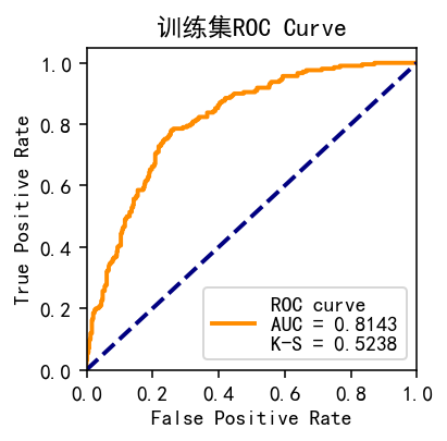
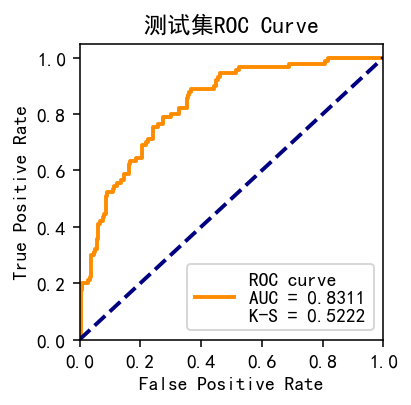
分别对比两种不同方式的效果

#statsmodels.api
plot_roc(target_train.values, resu_01,'训练集ROC Curve')  #训练集
plot_roc(target_test, resu_02,'测试集ROC Curve')

 

 使用perf_eva()函数对模型效果进行计算及可视化，基于预测的概率值和label值，提供KS(kolmogorov-smirnow), ROC, lift以及precision-recall四种评估指标：

#使用sc自带的
train_perf = sc.perf_eva(y_train, train_pred, title = "train")
test_perf = sc.perf_eva(y_test, test_pred, title = "test")

 

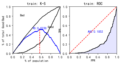
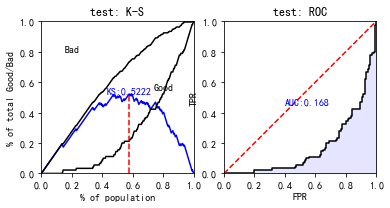
 这个auc看着好奇怪啊，估计是预测数据取预测good的概率，下面我们更改一下：

train_pred = lr.predict_proba(X_train)[:,0]
test_pred = lr.predict_proba(X_test)[:,0]
train_perf = sc.perf_eva(y_train, train_pred, title = "train")
test_perf = sc.perf_eva(y_test, test_pred, title = "test")

 

 现在数据就正常多了。

 

七、评分卡

scorecard()函数，生成的结果为各变量名及其分箱、对应得分组成的字典

def scorecard(bins, model, xcolumns, points0=600, odds0=1/19, 
              pdo=50, basepoints_eq0=False, digits=0)

各参数含义如下：

• bins：由`woebin`得到的分箱信息；
• model：LogisticRegression模型对象；
• points0：基准分数，默认值为600；
• odds0: 基准 Odds（好坏比），与真实违约概率对应，可换算得到违约概率，Odds = p/(1-p)。默认值为 1/19；
• pdo: Points toDouble theOdds，即Odds变成2倍时，所增加的信用分。默认值为50；
• basepoints_eq0：设置是否要把basepoints均分给每个变量的得分，默认为False，即不进行均分。但大多数评分卡倾向于所有分数均为正数，所以可手动改为True。

使用sklearn的逻辑回归这样转换

dat.creditability.value_counts(normalize=True)
'''
good    0.7
bad     0.3
'''
card = sc.scorecard(bins_adj, lr, X_train.columns,odds0=0.3/0.7)

使用statsmodels.api，则需要提供lr.coef_，lr.intercept_ 这两个系数

import numpy as np
result.intercept_ = np.array([result.params.const])
result.coef_ = np.array([result.params[1:].values])
card1 = sc.scorecard(bins_adj, result,model_cols,odds0=0.3/0.7)

转换之后，我们还需要验证，基础分为600，那么当分数等于600时候，逾期率就应该是0.3，本次使用toad的ks函数验证

#首先转换分数

#sc内置
train_score = sc.scorecard_ply(train, card, print_step=0)
test_score = sc.scorecard_ply(test, card, print_step=0)

import toad
t = toad.metrics.KS_bucket(train_score.iloc[:,0].values, target_train, bucket=10, method = 'quantile')

#statsmodels
train_score_01 = sc.scorecard_ply(train, card1, print_step=0)
test_score_01 = sc.scorecard_ply(test, card1, print_step=0)


t1 = toad.metrics.KS_bucket(train_score_01.iloc[:,0].values, target_train, bucket=10, method = 'quantile')

 

 

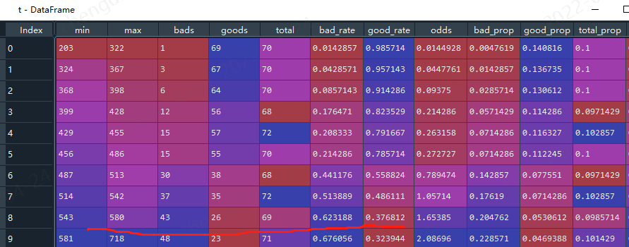
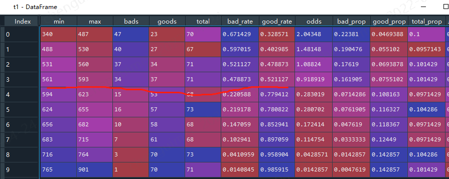
 使用sklearn的看着好变扭啊，最终是分数越高，逾期概率越高，

上面二者看着基本符合分数等于600时候，逾期率是0.3。

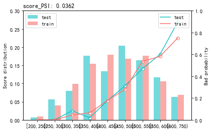
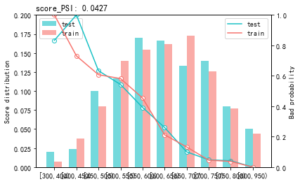
最后用perf_psi()得到该评分卡在测试数据集上的表现

#sc
sc.perf_psi(
  score = {'train':train_score, 'test':test_score},
  label = {'train':target_train, 'test':target_test}
)

#statsmodels
sc.perf_psi(
  score = {'train':train_score_01, 'test':test_score_01},
  label = {'train':target_train, 'test':target_test}
)