

XGBoost 学习调参的例子
发现后面设置参数的时候,原生接口和sklearn的参数混在一起了,现在修改为
def run_xgboost(data_x,data_y,random_state_num):
    train_x,valid_x,train_y,valid_y = train_test_split(data_x.values,data_y.values,test_size=0.25,random_state=random_state_num)
    print('开始训练模型')
    start = time.time()
    #转换成xgb运算格式
    d_train = xgb.DMatrix(train_x,train_y)
    d_valid = xgb.DMatrix(valid_x,valid_y)
    watchlist = [(d_train,'train'),(d_valid,'valid')]
    #参数设置(未调箱前的参数)
    params={
        'eta':0.2,                        #特征权重,取值范围0~1,通常最后设置eta为0.01~0.2
        'max_depth':3,                    #树的深度,通常取值3-10,过大容易过拟合,过小欠拟合
        'min_child_weight':1,             #最小样本的权重,调大参数可以繁殖过拟合
        'gamma':0.4,                      #控制是否后剪枝,越大越保守,一般0.1、 0.2的样子
        'subsample':0.8,                  #随机取样比例
        'colsample_bytree':0.8 ,          #默认为1,取值0~1,对特征随机采集比例
        'lambda':0.8,
        'alpha':0.6,
        'n_estimators':500,
        'booster':'gbtree',               #迭代树
        'objective':'binary:logistic',    #逻辑回归,输出为概率
        'nthread':6,                      #设置最大的进程量,若不设置则会使用全部资源
        'scale_pos_weight':1,             #默认为0,1可以处理类别不平衡

        'seed':1234,                      #随机树种子
        'silent':1,                       #0表示输出结果
        'eval_metric':'auc'               #评分指标
    }
    bst = xgb.train(params, d_train,1000,watchlist,early_stopping_rounds=100, verbose_eval=5)   #最大迭代次数1000次
    print(time.time()-start)
    tree_nums = bst.best_ntree_limit
    print('最优模型树的数量:%s,最优迭代次数:%s,auc: %s' %(bst.best_ntree_limit,bst.best_iteration,bst.best_score))
    bst = xgb.train(params, d_train,tree_nums,watchlist,early_stopping_rounds=100, verbose_eval=10) #最优模型迭代次数去训练

#     feat_imp = pd.Series(clf.booster().get_fscore()).sort_values(ascending=False)
#     #新版需要转换成dict or list
#     #feat_imp = pd.Series(dict(clf.get_booster().get_fscore())).sort_values(ascending=False)
#     #plt.bar(feat_imp.index, feat_imp)
#     feat_imp.plot(kind='bar', title='Feature Importances')
    #展示特征重要性排名
    feat_imp = bst.get_fscore(fmap='xgb.txt')
    feat_imp = sorted(feat_imp.items(),key=operator.itemgetter(1))
    df = pd.DataFrame(feat_imp,columns=['feature','fscore'])
    #每个特征被调用的次数/所有特征被调用总次数
    df['fscore'] = df['fscore']/df['fscore'].sum()
    #分数高的排在前面,展示前40个重要特征排名
    df = df.sort_values(by='fscore',ascending=False)
    df = df.iloc[:40]
    plt.figure()
    df.plot(kind='bar',x='feature',y='fscore',legend=True,figsize=(32,10))
    plt.title('XGBoost Feature Importance')
    plt.xlabel('relative importance')
    plt.gcf().savefig('feature_importance_xgb.png')
    plt.show()
    return bst
XGBoost 其实也是GBDT的一种,本编就说一下代码
导入模块
import numpy as np
import pandas as pd
import matplotlib.pyplot as plt
import operator
import time
import xgboost as xgb
from xgboost import plot_importance  #画特征重要性的函数
#from imblearn.ensemble import EasyEnsemble  #还有模块木有安装
from sklearn.model_selection import train_test_split
#from sklearn.externals import joblib 已经改成了下面这种方式
import joblib
from sklearn.metrics import auc,roc_curve  #说明是分类
plt.rc('font',family='SimHei',size=13)   #使画出的图形中能正常显示中文
%matplotlib inline
EDA数据探索性分析
#训练数据、线上数据(无Y)、验证数据
train_data = pd.read_csv('F:\\win10 升级桌面数据备份\\3.学习模型\\train_user_model_feat.csv')
print(len(train_data[train_data['label']==1]),len(train_data[train_data['label']==0]))  # 1: 815  0:42688
online_data = pd.read_csv('F:\\win10 升级桌面数据备份\\3.学习模型\\online_user_model_feat.csv')
valid_data = pd.read_csv('F:\\win10 升级桌面数据备份\\3.学习模型\\valid_user_model_feat.csv')
print(len(valid_data[valid_data['label']==1]),len(valid_data[valid_data['label']==0]))  # 1:892   0:39302
拆分特征和标签
train_y = train_data[['label']]
train_y.columns = ['y']
train_x = train_data.drop(['label','user_id'],axis=1)

valid_y = valid_data[['label']]
valid_y.columns = ['y']
valid_x = valid_data.drop(['label','user_id'],axis=1)
#
file_xgboost_model='./xgboost_model' #模型文件
file_xgboost_columns='./columns.csv' #最终使用的特征
file_xgboost_model_auc_ks='./xgboost_model_auc_ks.png' #模型AUC和KS值
file_xgboost_model_score='./xgboost_model_score.png' # 模型预测用户的评分分布
file_xgboost_model_prob='./xgboost_model_prob.png' #模型预测用户的概率分布
网格搜索法调参
#coding=utf-8
from xgboost import XGBClassifier
from sklearn.model_selection import GridSearchCV  #网格搜索法
import xgboost as xgb
def xgbpa(trainX, trainY):
    # init ,分类
    xgb1 = XGBClassifier(
        learning_rate=0.3,
        n_estimators=200,
        max_depth=5,
        min_child_weight=1,
        gamma=0,
        subsample=0.8,
        colsample_bytree=0.8,
        objective='binary:logistic',
        nthread=4,
        scale_pos_weight=1,
        seed=6
    )

    # max_depth 和 min_weight 参数调优   这个用给网格搜索法时的参数,数的层数由3-6
    param1 = {'max_depth': list(range(3, 7)), 'min_child_weight': list(range(1, 5, 2))}

    from sklearn import svm, datasets
    gsearch1 = GridSearchCV(
        estimator=XGBClassifier(
            learning_rate=0.3,
            n_estimators=150,
            max_depth=5,
            min_child_weight=1,
            gamma=0,
            subsample=0.8,
            colsample_bytree=0.8,
            objective='binary:logistic',
            nthread=4,
            scale_pos_weight=1,
            seed=6
        ),
        param_grid=param1, scoring='roc_auc', n_jobs=4, iid=False, cv=5)
    gsearch1.fit(trainX, trainY)
    print(gsearch1.scorer_)
    print(gsearch1.best_params_, gsearch1.best_score_)  #最佳参数(形式是字典型),最高分数(就一个值)
    best_max_depth = gsearch1.best_params_['max_depth'] #输出的max_depth的values
    best_min_child_weight = gsearch1.best_params_['min_child_weight']  #同理上面

    # gamma参数调优
    param2 = {'gamma': [i / 10.0 for i in range(0, 5, 2)]}
    gsearch2 = GridSearchCV(
        estimator=XGBClassifier(
            learning_rate=0.3,  # 如同学习率
            n_estimators=150,  # 树的个数
            max_depth=best_max_depth,  #同时替换上面的值
            min_child_weight=best_min_child_weight,  #同理上面
            gamma=0,
            subsample=0.8,
            colsample_bytree=0.8,
            objective='binary:logistic',
            nthread=4,
            scale_pos_weight=1,
            seed=6
        ),
        param_grid=param2, scoring='roc_auc', n_jobs=4, iid=False, cv=5)
    gsearch2.fit(trainX, trainY)
    print(gsearch2.scorer_)
    print(gsearch2.best_params_, gsearch2.best_score_)
    best_gamma = gsearch2.best_params_['gamma']

    # 调整subsample 和 colsample_bytree参数
    param3 = {'subsample': [i / 10.0 for i in range(6, 9)], 'colsample_bytree': [i / 10.0 for i in range(6, 9)]}
    gsearch3 = GridSearchCV(
        estimator=XGBClassifier(
            learning_rate=0.3,
            n_estimators=150,
            max_depth=best_max_depth,
            min_child_weight=best_min_child_weight,
            gamma=best_gamma,
            subsample=0.8,
            colsample_bytree=0.8,
            objective='binary:logistic',
            nthread=4,
            scale_pos_weight=1,
            seed=6
        ),
        param_grid=param3, scoring='roc_auc', n_jobs=4, iid=False, cv=5)
    gsearch3.fit(trainX, trainY)
    print(gsearch3.scorer_)
    print(gsearch3.best_params_, gsearch3.best_score_)
    best_subsample = gsearch3.best_params_['subsample']
    best_colsample_bytree = gsearch3.best_params_['colsample_bytree']

    # 正则化参数调优
    param4 = {'reg_alpha': [i / 10.0 for i in range(2, 10, 2)], 'reg_lambda': [i / 10.0 for i in range(2, 10, 2)]}
    gsearch4 = GridSearchCV(
        estimator=XGBClassifier(
            learning_rate=0.3,
            n_estimators=150,
            max_depth=best_max_depth,
            min_child_weight=best_min_child_weight,
            gamma=best_gamma,
            subsample=best_subsample,
            colsample_bytree=best_colsample_bytree,
            objective='binary:logistic',
            nthread=4,
            scale_pos_weight=1,
            seed=6
        ),
        param_grid=param4, scoring='roc_auc', n_jobs=4, iid=False, cv=5)
    gsearch4.fit(trainX, trainY)
    print(gsearch4.scorer_)
    print(gsearch4.best_params_, gsearch4.best_score_)
    best_reg_alpha = gsearch4.best_params_['reg_alpha']
    best_reg_lambda = gsearch4.best_params_['reg_lambda']


    param5= {'scale_pos_weight': [i for i in [0.5, 1, 2]]}

    gsearch5 = GridSearchCV(
        estimator = XGBClassifier(
            learning_rate = 0.3,
            n_estimators = 150,
            max_depth = best_max_depth,
            min_child_weight = best_min_child_weight,
            gamma = best_gamma,
            subsample = best_subsample,
            colsample_bytree = best_colsample_bytree,
            reg_alpha = best_reg_alpha,
            reg_lambda = best_reg_lambda,
            objective = 'binary:logistic',
            nthread = 4,
            scale_pos_weight = 1,
            seed = 6
            ),
        param_grid = param5, scoring = 'roc_auc', n_jobs = 4, iid = False, cv = 5)
    gsearch5.fit(trainX, trainY)
    print(gsearch5.best_params_, gsearch5.best_score_)
    best_scale_pos_weight = gsearch5.best_params_['scale_pos_weight']

    # 降低学习速率,数的数量
    param6 = [{'learning_rate': [0.01, 0.05, 0.1, 0.2], 'n_estimators': [800, 1000, 1200]}]

    gsearch6 = GridSearchCV(
        estimator=XGBClassifier(
            learning_rate=0.3,
            n_estimators=150,
            max_depth=best_max_depth,
            min_child_weight=best_min_child_weight,
            gamma=best_gamma,
            subsample=best_subsample,
            colsample_bytree=best_colsample_bytree,
            reg_alpha=best_reg_alpha,
            reg_lambda = best_reg_lambda,
            objective = 'binary:logistic',
            nthread = 4,
            scale_pos_weight = best_scale_pos_weight,
            seed = 6
    ),
    param_grid = param6, scoring = 'roc_auc', n_jobs = 4, iid = False, cv = 5)
    gsearch6.fit(trainX, trainY)
    print(gsearch6.scorer_)
    print(gsearch6.best_params_, gsearch6.best_score_)
    best_learning_rate = gsearch6.best_params_['learning_rate']
    best_n_estimators = gsearch6.best_params_['n_estimators']
    print('最好参数集:')
    print(gsearch1.best_params_, gsearch1.best_score_)
    print(gsearch2.best_params_, gsearch2.best_score_)
    print(gsearch3.best_params_, gsearch3.best_score_)
    print(gsearch4.best_params_, gsearch4.best_score_)
    print(gsearch5.best_params_, gsearch5.best_score_)
    print(gsearch6.best_params_, gsearch6.best_score_)


if __name__ == '__main__':
    # user_model cv
    #调参前得保持模型训练样本和调参样本数据一致
    print('--------------开始调参---------------')
    start = time.time()
    data_x,temp_x,data_y,temp_y = train_test_split(train_x,train_y,test_size=0.25,random_state=1234)
    xgbpa(data_x,data_y.y) #标签值有要是数组型的,不能是df,所以就.y了
    print('调参用时:%s'%(time.time()-start))
这个数据要跑挺久的(>0.5h)要留足时间去运行
--------------开始调参---------------
make_scorer(roc_auc_score, needs_threshold=True)
{'max_depth': 3, 'min_child_weight': 3} 0.8169763045780181
make_scorer(roc_auc_score, needs_threshold=True)
{'gamma': 0.0} 0.8169763045780181
make_scorer(roc_auc_score, needs_threshold=True)
{'colsample_bytree': 0.8, 'subsample': 0.8} 0.8169763045780181
make_scorer(roc_auc_score, needs_threshold=True)
{'reg_alpha': 0.6, 'reg_lambda': 0.8} 0.8148521719194484
{'scale_pos_weight': 0.5} 0.8155242908735241
make_scorer(roc_auc_score, needs_threshold=True)
{'learning_rate': 0.01, 'n_estimators': 1200} 0.8467294278425243
最好参数集:
{'max_depth': 3, 'min_child_weight': 3} 0.8169763045780181
{'gamma': 0.0} 0.8169763045780181
{'colsample_bytree': 0.8, 'subsample': 0.8} 0.8169763045780181
{'reg_alpha': 0.6, 'reg_lambda': 0.8} 0.8148521719194484
{'scale_pos_weight': 0.5} 0.8155242908735241
{'learning_rate': 0.01, 'n_estimators': 1200} 0.8467294278425243
调参用时:1126.5513534545898
特征列集索引表的建立
def create_feature_map(features):
    outfile = open('xgb.txt', 'w')  #写,新建一个叫xgb.txt的文件
    i = 0
    for feat in features:
        outfile.write('{0}\t{1}\tq\n'.format(i, feat))   #格式为 0  feature  q  \t是分隔符,为空  就是说第一列是序号,第二列是特征名称,第三列是q,不知道需要这个q干吗,可以是多写了,先要着吧,后面再看看吧
        i = i + 1
    outfile.close()
create_feature_map(train_x.columns)
使用XGBoost训练模型
只是用了一部分,还有一些参数没有根据最优参数来使用,但是大部分都已经运用进去了
#运行XGBoost,输出特征重要性排名
def run_xgboost(data_x,data_y,random_state_num):
    train_x,valid_x,train_y,valid_y = train_test_split(data_x.values,data_y.values,test_size=0.25,random_state=random_state_num)
    print('开始训练模型')
    start = time.time()
    #转换成xgb运算格式
    d_train = xgb.DMatrix(train_x,train_y)
    d_valid = xgb.DMatrix(valid_x,valid_y)
    watchlist = [(d_train,'train'),(d_valid,'valid')]
    #参数设置(未调箱前的参数)
    params={
        'eta':0.2,                        #特征权重,取值范围0~1,通常最后设置eta为0.01~0.2
        'max_depth':3,                    #树的深度,通常取值3-10,过大容易过拟合,过小欠拟合
        'min_child_weight':1,             #最小样本的权重,调大参数可以繁殖过拟合
        'gamma':0.4,                      #控制是否后剪枝,越大越保守,一般0.1、 0.2的样子
        'subsample':0.8,                  #随机取样比例
        'colsample_bytree':0.8 ,          #默认为1,取值0~1,对特征随机采集比例
        'reg_lambda':0.8,
        'reg_alpha':0.6,
        'learning_rate':0.1,
        'n_estimators':1000,
        'booster':'gbtree',               #迭代树
        'objective':'binary:logistic',    #逻辑回归,输出为概率
        'nthread':6,                      #设置最大的进程量,若不设置则会使用全部资源
        'scale_pos_weight':1,             #默认为0,1可以处理类别不平衡
        'lambda':1,                       #默认为1,用于L2平滑处理项,避免模型过拟合
        'seed':1234,                      #随机树种子
        'silent':1,                       #0表示输出结果
        'eval_metric':'auc'               #评分指标
    }
    bst = xgb.train(params, d_train,1000,watchlist,early_stopping_rounds=100, verbose_eval=5)   #最大迭代次数1000次
    print(time.time()-start)
    tree_nums = bst.best_ntree_limit
    print('最优模型树的数量:%s,最优迭代次数:%s,auc: %s' %(bst.best_ntree_limit,bst.best_iteration,bst.best_score))
    bst = xgb.train(params, d_train,tree_nums,watchlist,early_stopping_rounds=100, verbose_eval=10) #最优模型迭代次数去训练

#     feat_imp = pd.Series(clf.booster().get_fscore()).sort_values(ascending=False)
#     #新版需要转换成dict or list
#     #feat_imp = pd.Series(dict(clf.get_booster().get_fscore())).sort_values(ascending=False)
#     #plt.bar(feat_imp.index, feat_imp)
#     feat_imp.plot(kind='bar', title='Feature Importances')
    #展示特征重要性排名
    feat_imp = bst.get_fscore(fmap='xgb.txt')
    feat_imp = sorted(feat_imp.items(),key=operator.itemgetter(1))
    df = pd.DataFrame(feat_imp,columns=['feature','fscore'])
    #每个特征被调用的次数/所有特征被调用总次数
    df['fscore'] = df['fscore']/df['fscore'].sum()
    #分数高的排在前面,展示前40个重要特征排名
    df = df.sort_values(by='fscore',ascending=False)
    df = df.iloc[:40]
    plt.figure()
    df.plot(kind='bar',x='feature',y='fscore',legend=True,figsize=(32,10))
    plt.title('XGBoost Feature Importance')
    plt.xlabel('relative importance')
    plt.gcf().savefig('feature_importance_xgb.png')
    plt.show()
    return bst
绘制roc曲线函数
# 绘制ROC曲线函数
def plot_roc(test_x, test_y):
    predictions = bst.predict(xgb.DMatrix(test_x))
    false_positive_rate, true_positive_rate, thresholds = roc_curve(test_y, predictions)  #roc的几个参数
    roc_auc = auc(false_positive_rate, true_positive_rate)  #直接计算auc
    plt.title('Receiver Operating Characteristic')
    plt.plot(false_positive_rate,true_positive_rate, 'b', label='AUC = %0.4f' % roc_auc)
    plt.legend(loc='lower right')
    plt.plot([0, 1], [0, 1], 'r.')
    plt.xlim([0.0, 1.0])
    plt.ylim([0.0, 1.0])
    plt.ylabel('tpr')
    plt.xlabel('fpr')

# 绘制K-S函数 从大到小排序,分10等分
def plot_ks(test_x, test_y):
    predictions = bst.predict(xgb.DMatrix(test_x))
    false_positive_rate, true_positive_rate, thresholds = roc_curve(test_y, predictions, drop_intermediate=False)
    pre = sorted(predictions, reverse=True)  #reverse参数为True意味着按照降序排序,这是画ks时要求的
    num = []
    for i in range(10):
        num.append((i) * int(len(pre) / 10))
    num.append(len(pre) - 1)
    df = pd.DataFrame()
    df['false_positive_rate'] = false_positive_rate
    df['true_positive_rate'] = true_positive_rate
    df['thresholds'] = thresholds
    data_ks = []
    for i in num:
        data_ks.append(list(df[df['thresholds'] == pre[i]].values[0]))
    data_ks = pd.DataFrame(data_ks)
    data_ks.columns = ['fpr', 'tpr', 'thresholds']
    ks = max(data_ks['tpr'] - data_ks['fpr'])
    plt.title('K-S曲线')
    plt.plot(np.array(range(len(num))), data_ks['tpr'])
    plt.plot(np.array(range(len(num))), data_ks['fpr'])
    plt.plot(np.array(range(len(num))), data_ks['tpr'] - data_ks['fpr'], label='K-S = %0.4f' % ks)
    plt.legend(loc='lower right')
    plt.xlim([0, 10])
    plt.ylim([0.0, 1.0])
    plt.ylabel('累计占比')
    plt.xlabel('分组编号')

# 绘制一张图,包含训练和测试集的ROC、AUC、K-S图形指标。
def auc_ks(train_x, test_x, train_y, test_y):
    plt.figure(figsize=(15, 15))
    plt.subplot(221)
    plot_roc(train_x, train_y)
    plt.subplot(222)
    plot_roc(test_x, test_y)
    plt.subplot(223)
    plot_ks(train_x, train_y)
    plt.subplot(224)
    plot_ks(test_x, test_y)
    plt.savefig(file_xgboost_model_auc_ks)
    plt.show()
保存模型、评价指标、选择变量等
#保存模型、评价指标、选择变量到D盘
def run_main(data_x,data_y):
    global bst
    start=time.time()
    bst=run_xgboost(data_x,data_y,random_state_num=1234)  #为什么要是1234,因为调参时候就是=1234
    joblib.dump(bst, file_xgboost_model)  #joblib的用法https://www.cnblogs.com/wzdLY/p/9630671.html 将模型保存
    print('模型已成功保存在 %s'%(file_xgboost_model))
    train_x, test_x, train_y, test_y = train_test_split(data_x.values, data_y.values, test_size=0.25, random_state=1234)
    auc_ks(train_x, test_x, train_y, test_y)
    print('模型评价指标已保存在:%s'%(file_xgboost_model_auc_ks))
    print('运行共花费时间:%s'%(time.time()-start))

if __name__=='__main__':
    run_main(train_x, train_y)
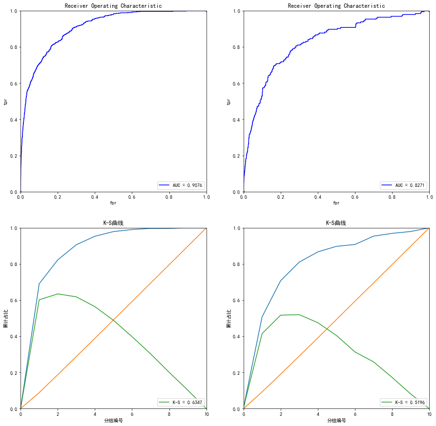

分别是训练集和测试集的auc和ks,还有特征重要性的排列
用验证集数据验证模型效果
# 绘制ROC曲线函数
def plot_test_roc(test_x, test_y,filename):
    bst = joblib.load(filename)
    predictions = bst.predict(xgb.DMatrix(test_x.values))
    false_positive_rate,true_positive_rate, thresholds = roc_curve(test_y, predictions)
    roc_auc = auc(false_positive_rate, true_positive_rate)
    plt.title('Receiver Operating Characteristic')
    plt.plot(false_positive_rate,true_positive_rate, 'b', label='AUC = %0.4f' % roc_auc)
    plt.legend(loc='lower right')
    plt.plot([0, 1], [0, 1], 'r--')
    plt.xlim([0.0, 1.0])
    plt.ylim([0.0, 1.0])
    plt.ylabel('Recall')
    plt.xlabel('Fall-out')
    plt.show()

if __name__=='__main__':
    plot_test_roc(valid_x,valid_y,file_xgboost_model)

下面附上全部代码


# -*- coding: utf-8 -*-
"""
Created on Wed Mar 10 19:01:07 2021

@author: Administrator
"""


#%%
import numpy as np
import pandas as pd
import matplotlib.pyplot as plt
import operator
import time
import xgboost as xgb
from xgboost import plot_importance  #画特征重要性的函数
#from imblearn.ensemble import EasyEnsemble  #还有模块木有安装
from sklearn.model_selection import train_test_split
#from sklearn.externals import joblib 已经改成了下面这种方式
import joblib
from sklearn.metrics import auc,roc_curve  #说明是分类
plt.rc('font',family='SimHei',size=13)   #使画出的图形中能正常显示中文
%matplotlib inline


#%%
#训练数据、线上数据(无Y)、验证数据
train_data = pd.read_csv('D:/迅雷下载/3.学习模型/3.学习模型/train_user_model_feat.csv')
print(len(train_data[train_data['label']==1]),len(train_data[train_data['label']==0]))  # 1: 815  0:42688
online_data = pd.read_csv('D:/迅雷下载/3.学习模型/3.学习模型/online_user_model_feat.csv')
valid_data = pd.read_csv('D:/迅雷下载/3.学习模型/3.学习模型/valid_user_model_feat.csv')
print(len(valid_data[valid_data['label']==1]),len(valid_data[valid_data['label']==0]))  # 1:892   0:39302


#%%
train_y = train_data[['label']]
train_y.columns = ['y']
train_x = train_data.drop(['label','user_id'],axis=1)

valid_y = valid_data[['label']]
valid_y.columns = ['y']
valid_x = valid_data.drop(['label','user_id'],axis=1)
#
file_xgboost_model='./xgboost_model' #模型文件
file_xgboost_columns='./columns.csv' #最终使用的特征
file_xgboost_model_auc_ks='./xgboost_model_auc_ks.png' #模型AUC和KS值
file_xgboost_model_score='./xgboost_model_score.png' # 模型预测用户的评分分布
file_xgboost_model_prob='./xgboost_model_prob.png' #模型预测用户的概率分布


#%%
#coding=utf-8
from xgboost import XGBClassifier
from sklearn.model_selection import GridSearchCV  #网格搜索法
import xgboost as xgb
def xgbpa(trainX, trainY):
    # init ,分类
    xgb1 = XGBClassifier(
        learning_rate=0.3,
        n_estimators=150,
        max_depth=5,
        min_child_weight=1,
        gamma=0,
        subsample=0.8,
        colsample_bytree=0.8,
        objective='binary:logistic',
        nthread=4,
        scale_pos_weight=1,
        seed=6
    )

    # max_depth 和 min_weight 参数调优   这个用给网格搜索法时的参数,数的层数由3-6
    param1 = {'max_depth': list(range(3, 7)), 'min_child_weight': list(range(1, 5, 2))}

    from sklearn import svm, datasets
    gsearch1 = GridSearchCV(
        estimator=XGBClassifier(
            learning_rate=0.3,
            n_estimators=150,
            max_depth=5,
            min_child_weight=1,
            gamma=0,
            subsample=0.8,
            colsample_bytree=0.8,
            objective='binary:logistic',
            nthread=4,
            scale_pos_weight=1,
            seed=6
        ),
        param_grid=param1, scoring='roc_auc', n_jobs=4, iid=False, cv=5)
    gsearch1.fit(trainX, trainY)
    print(gsearch1.scorer_)
    print(gsearch1.best_params_, gsearch1.best_score_)  #最佳参数(形式是字典型),最高分数(就一个值)
    best_max_depth = gsearch1.best_params_['max_depth'] #输出的max_depth的values
    best_min_child_weight = gsearch1.best_params_['min_child_weight']  #同理上面

    # gamma参数调优
    param2 = {'gamma': [i / 10.0 for i in range(0, 5, 2)]}
    gsearch2 = GridSearchCV(
        estimator=XGBClassifier(
            learning_rate=0.3,  # 如同学习率
            n_estimators=150,  # 树的个数
            max_depth=best_max_depth,  #同时替换上面的值
            min_child_weight=best_min_child_weight,  #同理上面
            gamma=0,
            subsample=0.8,
            colsample_bytree=0.8,
            objective='binary:logistic',
            nthread=4,
            scale_pos_weight=1,
            seed=6
        ),
        param_grid=param2, scoring='roc_auc', n_jobs=4, iid=False, cv=5)
    gsearch2.fit(trainX, trainY)
    print(gsearch2.scorer_)
    print(gsearch2.best_params_, gsearch2.best_score_)
    best_gamma = gsearch2.best_params_['gamma']

    # 调整subsample 和 colsample_bytree参数
    param3 = {'subsample': [i / 10.0 for i in range(6, 9)], 'colsample_bytree': [i / 10.0 for i in range(6, 9)]}
    gsearch3 = GridSearchCV(
        estimator=XGBClassifier(
            learning_rate=0.3,
            n_estimators=150,
            max_depth=best_max_depth,
            min_child_weight=best_min_child_weight,
            gamma=best_gamma,
            subsample=0.8,
            colsample_bytree=0.8,
            objective='binary:logistic',
            nthread=4,
            scale_pos_weight=1,
            seed=6
        ),
        param_grid=param3, scoring='roc_auc', n_jobs=4, iid=False, cv=5)
    gsearch3.fit(trainX, trainY)
    print(gsearch3.scorer_)
    print(gsearch3.best_params_, gsearch3.best_score_)
    best_subsample = gsearch3.best_params_['subsample']
    best_colsample_bytree = gsearch3.best_params_['colsample_bytree']

    # 正则化参数调优
    param4 = {'reg_alpha': [i / 10.0 for i in range(2, 10, 2)], 'reg_lambda': [i / 10.0 for i in range(2, 10, 2)]}
    gsearch4 = GridSearchCV(
        estimator=XGBClassifier(
            learning_rate=0.3,
            n_estimators=150,
            max_depth=best_max_depth,
            min_child_weight=best_min_child_weight,
            gamma=best_gamma,
            subsample=best_subsample,
            colsample_bytree=best_colsample_bytree,
            objective='binary:logistic',
            nthread=4,
            scale_pos_weight=1,
            seed=6
        ),
        param_grid=param4, scoring='roc_auc', n_jobs=4, iid=False, cv=5)
    gsearch4.fit(trainX, trainY)
    print(gsearch4.scorer_)
    print(gsearch4.best_params_, gsearch4.best_score_)
    best_reg_alpha = gsearch4.best_params_['reg_alpha']
    best_reg_lambda = gsearch4.best_params_['reg_lambda']


    param5= {'scale_pos_weight': [i for i in [0.5, 1, 2]]}

    gsearch5 = GridSearchCV(
        estimator = XGBClassifier(
            learning_rate = 0.3,
            n_estimators = 150,
            max_depth = best_max_depth,
            min_child_weight = best_min_child_weight,
            gamma = best_gamma,
            subsample = best_subsample,
            colsample_bytree = best_colsample_bytree,
            reg_alpha = best_reg_alpha,
            reg_lambda = best_reg_lambda,
            objective = 'binary:logistic',
            nthread = 4,
            scale_pos_weight = 1,
            seed = 6
            ),
        param_grid = param5, scoring = 'roc_auc', n_jobs = 4, iid = False, cv = 5)
    gsearch5.fit(trainX, trainY)
    print(gsearch5.best_params_, gsearch5.best_score_)
    best_scale_pos_weight = gsearch5.best_params_['scale_pos_weight']

    # 降低学习速率,数的数量
    param6 = [{'learning_rate': [0.01, 0.05, 0.1, 0.2], 'n_estimators': [800, 1000, 1200]}]

    gsearch6 = GridSearchCV(
        estimator=XGBClassifier(
            learning_rate=0.3,
            n_estimators=150,
            max_depth=best_max_depth,
            min_child_weight=best_min_child_weight,
            gamma=best_gamma,
            subsample=best_subsample,
            colsample_bytree=best_colsample_bytree,
            reg_alpha=best_reg_alpha,
            reg_lambda = best_reg_lambda,
            objective = 'binary:logistic',
            nthread = 4,
            scale_pos_weight = best_scale_pos_weight,
            seed = 6
    ),
    param_grid = param6, scoring = 'roc_auc', n_jobs = 4, iid = False, cv = 5)
    gsearch6.fit(trainX, trainY)
    print(gsearch6.scorer_)
    print(gsearch6.best_params_, gsearch6.best_score_)
    best_learning_rate = gsearch6.best_params_['learning_rate']
    best_n_estimators = gsearch6.best_params_['n_estimators']
    print('最好参数集:')
    print(gsearch1.best_params_, gsearch1.best_score_)
    print(gsearch2.best_params_, gsearch2.best_score_)
    print(gsearch3.best_params_, gsearch3.best_score_)
    print(gsearch4.best_params_, gsearch4.best_score_)
    print(gsearch5.best_params_, gsearch5.best_score_)
    print(gsearch6.best_params_, gsearch6.best_score_)


if __name__ == '__main__':
    # user_model cv
    #调参前得保持模型训练样本和调参样本数据一致
    print('--------------开始调参---------------')
    start = time.time()
    data_x,temp_x,data_y,temp_y = train_test_split(train_x,train_y,test_size=0.25,random_state=1234)
    xgbpa(data_x,data_y.y) #标签值有要是数组型的,不能是df,所以就.y了
    print('调参用时:%s'%(time.time()-start))

#%%
def create_feature_map(features):
    outfile = open('xgb.txt', 'w')  #写,新建一个叫xgb.txt的文件
    i = 0
    for feat in features:
        outfile.write('{0}\t{1}\tq\n'.format(i, feat))   #格式为 0  feature  q  \t是分隔符,为空  就是说第一列是序号,第二列是特征名称,第三列是q,不知道需要这个q干吗,可以是多写了,先要着吧,后面再看看吧
        i = i + 1
    outfile.close()
create_feature_map(train_x.columns)

#%%
#运行XGBoost,输出特征重要性排名
def run_xgboost(data_x,data_y,random_state_num):
    train_x,valid_x,train_y,valid_y = train_test_split(data_x.values,data_y.values,test_size=0.25,random_state=random_state_num)
    print('开始训练模型')
    start = time.time()
    #转换成xgb运算格式
    d_train = xgb.DMatrix(train_x,train_y)
    d_valid = xgb.DMatrix(valid_x,valid_y)
    watchlist = [(d_train,'train'),(d_valid,'valid')]
    #参数设置(未调箱前的参数)
    params={
        'eta':0.2,                        #特征权重,取值范围0~1,通常最后设置eta为0.01~0.2
        'max_depth':3,                    #树的深度,通常取值3-10,过大容易过拟合,过小欠拟合
        'min_child_weight':1,             #最小样本的权重,调大参数可以繁殖过拟合
        'gamma':0.4,                      #控制是否后剪枝,越大越保守,一般0.1、 0.2的样子
        'subsample':0.8,                  #随机取样比例
        'colsample_bytree':0.8 ,          #默认为1,取值0~1,对特征随机采集比例
        'reg_lambda':0.8,
        'reg_alpha':0.6,
        'learning_rate':0.1,
        'n_estimators':1000,
        'booster':'gbtree',               #迭代树
        'objective':'binary:logistic',    #逻辑回归,输出为概率
        'nthread':6,                      #设置最大的进程量,若不设置则会使用全部资源
        'scale_pos_weight':1,             #默认为0,1可以处理类别不平衡
        'lambda':1,                       #默认为1,用于L2平滑处理项,避免模型过拟合
        'seed':1234,                      #随机树种子
        'silent':1,                       #0表示输出结果
        'eval_metric':'auc'               #评分指标
    }
    bst = xgb.train(params, d_train,1000,watchlist,early_stopping_rounds=100, verbose_eval=5)   #最大迭代次数1000次
    print(time.time()-start)
    tree_nums = bst.best_ntree_limit
    print('最优模型树的数量:%s,最优迭代次数:%s,auc: %s' %(bst.best_ntree_limit,bst.best_iteration,bst.best_score))
    bst = xgb.train(params, d_train,tree_nums,watchlist,early_stopping_rounds=100, verbose_eval=10) #最优模型迭代次数去训练

#     feat_imp = pd.Series(clf.booster().get_fscore()).sort_values(ascending=False)
#     #新版需要转换成dict or list
#     #feat_imp = pd.Series(dict(clf.get_booster().get_fscore())).sort_values(ascending=False)
#     #plt.bar(feat_imp.index, feat_imp)
#     feat_imp.plot(kind='bar', title='Feature Importances')
    #展示特征重要性排名
    feat_imp = bst.get_fscore(fmap='xgb.txt')
    feat_imp = sorted(feat_imp.items(),key=operator.itemgetter(1))
    df = pd.DataFrame(feat_imp,columns=['feature','fscore'])
    #每个特征被调用的次数/所有特征被调用总次数
    df['fscore'] = df['fscore']/df['fscore'].sum()
    #分数高的排在前面,展示前40个重要特征排名
    df = df.sort_values(by='fscore',ascending=False)
    df = df.iloc[:40]
    plt.figure()
    df.plot(kind='bar',x='feature',y='fscore',legend=True,figsize=(32,10))
    plt.title('XGBoost Feature Importance')
    plt.xlabel('relative importance')
    plt.gcf().savefig('feature_importance_xgb.png')
    plt.show()
    return bst

#%%
# 绘制ROC曲线函数
def plot_roc(test_x, test_y):
    predictions = bst.predict(xgb.DMatrix(test_x))
    false_positive_rate, true_positive_rate, thresholds = roc_curve(test_y, predictions)  #roc的几个参数
    roc_auc = auc(false_positive_rate, true_positive_rate)  #直接计算auc
    plt.title('Receiver Operating Characteristic')
    plt.plot(false_positive_rate,true_positive_rate, 'b', label='AUC = %0.4f' % roc_auc)
    plt.legend(loc='lower right')
    plt.plot([0, 1], [0, 1], 'r.')
    plt.xlim([0.0, 1.0])
    plt.ylim([0.0, 1.0])
    plt.ylabel('tpr')
    plt.xlabel('fpr')

# 绘制K-S函数 从大到小排序,分10等分
def plot_ks(test_x, test_y):
    predictions = bst.predict(xgb.DMatrix(test_x))
    false_positive_rate, true_positive_rate, thresholds = roc_curve(test_y, predictions, drop_intermediate=False)
    pre = sorted(predictions, reverse=True)  #reverse参数为True意味着按照降序排序,这是画ks时要求的
    num = []
    for i in range(10):
        num.append((i) * int(len(pre) / 10))
    num.append(len(pre) - 1)
    df = pd.DataFrame()
    df['false_positive_rate'] = false_positive_rate
    df['true_positive_rate'] = true_positive_rate
    df['thresholds'] = thresholds
    data_ks = []
    for i in num:
        data_ks.append(list(df[df['thresholds'] == pre[i]].values[0]))
    data_ks = pd.DataFrame(data_ks)
    data_ks.columns = ['fpr', 'tpr', 'thresholds']
    ks = max(data_ks['tpr'] - data_ks['fpr'])
    plt.title('K-S曲线')
    plt.plot(np.array(range(len(num))), data_ks['tpr'])
    plt.plot(np.array(range(len(num))), data_ks['fpr'])
    plt.plot(np.array(range(len(num))), data_ks['tpr'] - data_ks['fpr'], label='K-S = %0.4f' % ks)
    plt.legend(loc='lower right')
    plt.xlim([0, 10])
    plt.ylim([0.0, 1.0])
    plt.ylabel('累计占比')
    plt.xlabel('分组编号')

# 绘制一张图,包含训练和测试集的ROC、AUC、K-S图形指标。
def auc_ks(train_x, test_x, train_y, test_y):
    plt.figure(figsize=(15, 15))
    plt.subplot(221)
    plot_roc(train_x, train_y)
    plt.subplot(222)
    plot_roc(test_x, test_y)
    plt.subplot(223)
    plot_ks(train_x, train_y)
    plt.subplot(224)
    plot_ks(test_x, test_y)
    plt.savefig(file_xgboost_model_auc_ks)
    plt.show()

#%%
#保存模型、评价指标、选择变量到D盘
def run_main(data_x,data_y):
    global bst
    start=time.time()
    bst=run_xgboost(data_x,data_y,random_state_num=1234)  #为什么要是1234,因为调参时候就是=1234
    joblib.dump(bst, file_xgboost_model)  #joblib的用法https://www.cnblogs.com/wzdLY/p/9630671.html 将模型保存
    print('模型已成功保存在 %s'%(file_xgboost_model))
    train_x, test_x, train_y, test_y = train_test_split(data_x.values, data_y.values, test_size=0.25, random_state=1234)
    auc_ks(train_x, test_x, train_y, test_y)
    print('模型评价指标已保存在:%s'%(file_xgboost_model_auc_ks))
    print('运行共花费时间:%s'%(time.time()-start))

if __name__=='__main__':
    run_main(train_x, train_y)

# 绘制ROC曲线函数
def plot_test_roc(test_x, test_y,filename):
    bst = joblib.load(filename)
    predictions = bst.predict(xgb.DMatrix(test_x.values))
    false_positive_rate,true_positive_rate, thresholds = roc_curve(test_y, predictions)
    roc_auc = auc(false_positive_rate, true_positive_rate)
    plt.title('Receiver Operating Characteristic')
    plt.plot(false_positive_rate,true_positive_rate, 'b', label='AUC = %0.4f' % roc_auc)
    plt.legend(loc='lower right')
    plt.plot([0, 1], [0, 1], 'r--')
    plt.xlim([0.0, 1.0])
    plt.ylim([0.0, 1.0])
    plt.ylabel('Recall')
    plt.xlabel('Fall-out')
    plt.show()

if __name__=='__main__':
    plot_test_roc(valid_x,valid_y,file_xgboost_model)
这里主要补充一下这个调参的不足之处
1.调参使用的是全部样本,这样不是很适合
2.使用网格搜索法,太耗时,
3.调参顺序不对,最后面的效果不好
后面我又使用逻辑回归做了一个模型,代码如下:
# -*- coding: utf-8 -*-
"""
Created on Wed Mar 10 15:58:41 2021

@author: Administrator
"""

#%%
import numpy as np
import pandas as pd
import matplotlib.pyplot as plt
import operator
import time
import xgboost as xgb
from xgboost import plot_importance  #画特征重要性的函数
#from imblearn.ensemble import EasyEnsemble  #还有模块木有安装
from sklearn.model_selection import train_test_split
#from sklearn.externals import joblib 已经改成了下面这种方式
import joblib
from sklearn.metrics import auc,roc_curve  #说明是分类
plt.rc('font',family='SimHei',size=13)   #使画出的图形中能正常显示中文
%matplotlib inline


#%%
#训练数据、线上数据(无Y)、验证数据
train_data = pd.read_csv('D:/迅雷下载/3.学习模型/3.学习模型/train_user_model_feat.csv')
print(len(train_data[train_data['label']==1]),len(train_data[train_data['label']==0]))  # 1: 815  0:42688
online_data = pd.read_csv('D:/迅雷下载/3.学习模型/3.学习模型/online_user_model_feat.csv')
valid_data = pd.read_csv('D:/迅雷下载/3.学习模型/3.学习模型/valid_user_model_feat.csv')
print(len(valid_data[valid_data['label']==1]),len(valid_data[valid_data['label']==0]))  # 1:892   0:39302


#%%
for i in train_data.columns :
    print(i,train_data[i].nunique())
a=[]
for i in train_data.columns :
    if train_data[i].nunique()<10:
        a.append(i)
a=['rule_uid',
 'user_lv_cd',
 'user_date_cnt_b7day',
 'uc_date_cnt_b7day',
 'uc_act_4',
 'uc_buy_bool_day7']

train_data.pop('user_id')
train_data['y'] = train_data['label']
train_data.pop('label')

#%%类别型变量的iv
import pycard as pc
cate_iv_woedf = pc.WoeDf()
for i in a:
    cate_iv_woedf.append(pc.cross_woe(train_data[i] ,train_data.y))
#cate_iv_woedf.to_excel('tmp1')

#%%数值型变量的iv
num_col = [i for i in train_data.columns if i not in a]
num_col.remove('y')
clf = pc.NumBin(min_bin_samples=200, min_impurity_decrease=4e-5)
for i in num_col:
    clf.fit(train_data[i] ,train_data.y)
    #clf.generate_transform_fun()
    cate_iv_woedf.append(clf.woe_df_)


#%%相关性分析
train_data.corr_tri().abs().to_excel('tmp1.xlsx')

def argmax(x):
    """计算 df 的最大值所对应的行、列索引,返回 (row, cols) 元组"""
    m0 = x.max()
    max_value = m0.max()
    col_label = m0.idxmax()
    row_label = x[col_label].idxmax()
    return row_label, col_label


def corr_filter(detail_df, vars_iv, corr_tol=0.9, iv_diff=0.01):
    """相关性系数 >= tol的两个列, 假设 var1 的 IV 比 var2 的 IV 更高:
        若 var1_iv - var2_iv > iv_diff,则将其中 IV 值更低的列删除 \n

    参数:
    ----------
    detail_sr: dataframe, 需要计算相关性的明细数据框 \n
    vars_iv: dataframe, 包含2列:colName和iv列。各个变量的 IV 指标
        该参数的值一般由 woedf.var_ivs 方法返回。 \n
    corr_tol: float, 线性相关性阈值,超过此阈值的两个列,则判断两个列相关性过高,进而判断 IV 之差是否足够大 \n
    iv_diff: float, 两个列的 IV 差值的阈值,自动删除 IV 更低的列

    返回值:
    ----------
    corr_df: dataframe, 相关性矩阵,并删除了相关性超过阈值的列 \n
    dropped_col: list, 删除的列"""
    corr_df = detail_df.corr_tri().abs()
    vars_iv = vars_iv.set_index('colName')
    corr_df = corr_df.fillna(0)
    dropped_col = []
    while True:
        row, col = argmax(corr_df)
        if corr_df.loc[row, col] >= corr_tol:
            drop_label = row if vars_iv.loc[row,'IV'] < vars_iv.loc[col,'IV'] else col
            dropped_col.append(drop_label)
            corr_df = corr_df.drop(drop_label).drop(drop_label, axis=1)
            vars_iv = vars_iv.drop(drop_label)
            if len(corr_df) == 1:
                break
        else:
            break
    return corr_df, dropped_col
t=cate_iv_woedf.var_ivs().iloc[:,0:-1].reset_index()
t.columns = ['colName','IV']
corr_df, dropped_col = corr_filter(train_data[a+num_col],t,corr_tol=0.75, iv_diff=0.00001)

data_drop_corr = train_data.drop(columns = dropped_col)

#%%
cate_iv_woedf = pc.WoeDf()
clf = pc.NumBin(min_bin_samples=200, min_impurity_decrease=4e-5)
for i in data_drop_corr.columns:
    clf.fit(data_drop_corr[i] ,data_drop_corr.y)
    #clf.generate_transform_fun()
    cate_iv_woedf.append(clf.woe_df_)

cate_iv_woedf.to_excel('tmp1')


#%%删除下面这些字段
drop_2 = ["uc_date_cnt_b7day",
"user_act_totalCnt_15day",
"max_click",
"freq_click",
"uc_act_decay_3",
"uc_act_4",
"uc_act_time_zone_0",
"uc_act_time_zone_1",
"ratio_1_6",
"uc_last_tm_dist",
"user_date_cnt_b15day",
"uc_date_cnt_b15day",
"uc_date_ratio_15",
"uc_act_totalCnt",
"uc_act_ratio_60day",
"uc_act_ratio_15day",
"ratio_act_time_1day",
"user_act_time_5day",
"ratio_act_time_5day",
"mean_uc_act",
"uc_act_time_zone_2",
"uc_act_time_zone_3",
"uc_buy_bool_day7"]

# 去掉这些V13    V15    V22    V24    V25    V26
num_col = [i for i in data_drop_corr.columns if i not in drop_2]
num_col.remove('y')

num_iv_woedf = pc.WoeDf()
clf = pc.NumBin(min_bin_samples=200, min_impurity_decrease=4e-5)
for i in num_col:
    clf.fit(data_drop_corr[i] ,data_drop_corr.y)
    data_drop_corr[i+'_bin'] = clf.transform(data_drop_corr[i])  #这样可以省略掉后面转换成_bin的一步骤
    num_iv_woedf.append(clf.woe_df_)


#%%woe转换
bin_col = [i for i in list(data_drop_corr.columns) if i[-4:]=='_bin']

cate_iv_woedf = pc.WoeDf()
for i in bin_col:
    cate_iv_woedf.append(pc.cross_woe(data_drop_corr[i] ,data_drop_corr.y))
#cate_iv_woedf.to_excel('tmp1')
cate_iv_woedf.bin2woe(data_drop_corr,bin_col)
cate_iv_woedf.to_excel('tmp.xlsx')

#%%建模
model_col = [i for i in list(data_drop_corr.columns) if i[-4:]=='_woe']

import pandas as pd
import matplotlib.pyplot as plt #导入图像库
import matplotlib
import seaborn as sns
import statsmodels.api as sm
from sklearn.metrics import roc_curve, auc
from sklearn.model_selection import train_test_split

X = data_drop_corr[model_col]
Y = data_drop_corr['y']


x_train,x_test,y_train,y_test=train_test_split(X,Y,test_size=0.3,random_state=100)


X1=sm.add_constant(x_train)   #在X前加上一列常数1,方便做带截距项的回归
logit=sm.Logit(y_train.astype(float),X1.astype(float))
result=logit.fit()
result.summary()
result.params

resu_1 = result.predict(X1.astype(float))
fpr, tpr, threshold = roc_curve(y_train, resu_1)
rocauc = auc(fpr, tpr)  #0.9693313248601317
plt.plot(fpr, tpr, 'b', label='AUC = %0.2f' % rocauc)
plt.legend(loc='lower right')
plt.plot([0, 1], [0, 1], 'r--')
plt.xlim([0, 1])
plt.ylim([0, 1])
plt.ylabel('真正率')
plt.xlabel('假正率')
plt.show()


#%%测试集
X3 = sm.add_constant(x_test)
resu = result.predict(X3.astype(float))
fpr, tpr, threshold = roc_curve(y_test, resu)
rocauc = auc(fpr, tpr)
plt.plot(fpr, tpr, 'b', label='AUC = %0.2f' % rocauc)
plt.legend(loc='lower right')
plt.plot([0, 1], [0, 1], 'r--')
plt.xlim([0, 1])
plt.ylim([0, 1])
plt.ylabel('真正率')
plt.xlabel('假正率')
plt.show()

#%%验证集

num_iv_woedf_1 = pc.WoeDf()
clf = pc.NumBin(min_bin_samples=200, min_impurity_decrease=4e-5)
for i in num_col:
    clf.fit(data_drop_corr[i] ,data_drop_corr.y)
    valid_data[i+'_bin'] = pc.binning(valid_data[i],clf.bins_) #这样可以省略掉后面转换成_bin的一步骤
    #num_iv_woedf_1.append(clf.woe_df_)

#%%woe转换
bin_col_1 = [i for i in list(valid_data.columns) if i[-4:]=='_bin']

cate_iv_woedf.bin2woe(valid_data,bin_col)
model_col_1 = [i for i in list(valid_data.columns) if i[-4:]=='_woe']

valid_data = valid_data.rename(columns={'label':'y'})
X_test = valid_data[model_col_1]
Y_test = valid_data['y']


X4 = sm.add_constant(X_test)
resu = result.predict(X4.astype(float))
fpr, tpr, threshold = roc_curve(Y_test, resu)
rocauc = auc(fpr, tpr)  #0.7931891609482327
plt.plot(fpr, tpr, 'b', label='AUC = %0.2f' % rocauc)
plt.legend(loc='lower right')
plt.plot([0, 1], [0, 1], 'r--')
plt.xlim([0, 1])
plt.ylim([0, 1])
plt.ylabel('真正率')
plt.xlabel('假正率')
plt.show()

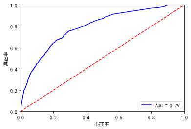
上面分别是测试集和验证集的auc ,比xgboost的验证集差一点,但是测试集比他好一点,这也验证了xgboost不易过拟合的性质

 浙公网安备 33010602011771号