
sklearn.model_selection
划分数据集方法:
- 留出法(train_test_split)
- 交叉验证法
- KFold方法 k折交叉验证
- RepeatedKFold p次k折交叉验证
- LeaveOneOut 留一法
- LeavePOut 留P法
- ShuffleSplit 随机分配
- 自助法
一、留出法
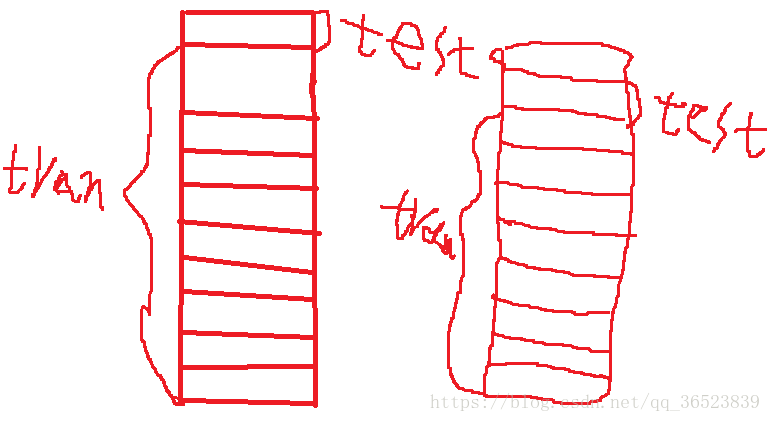
留出法的想法很简单,将原始数据直接划分为互斥的两类,其中一部分用来训练模型,另外一部分用来测试。前者就是训练集,后者就是测试集。
在sklearn当中,使用train_test_split可以将数据分为训练集和测试集
补充一下train_test_split的stratify参数:
stratify是为了保持split前类的分布。比如有100个数据,80个属于A类,20个属于B类。如果train_test_split(... test_size=0.25, stratify = y_all), 那么split之后数据如下:
training: 75个数据,其中60个属于A类,15个属于B类。
testing: 25个数据,其中20个属于A类,5个属于B类。
用了stratify参数,training集和testing集的类的比例是 A:B= 4:1,等同于split前的比例(80:20)。通常在这种类分布不平衡的情况下会用到stratify。
将stratify=X就是按照X中的比例分配
将stratify=y就是按照y中的比例分配
#官方示例,使用鸢尾花的数据集
import numpy as np
from sklearn.datasets  import load_iris
from sklearn import svm #支持向量机
from sklearn.model_selection import train_test_split

x,y=load_iris(return_X_y=True)
x_train,x_test,y_train,y_test=train_test_split(x,y,test_size=0.4,random_state=0)
x_train.shape,y_train.shape
clf=svm.SVC(kernel='linear',C=1).fit(x_train,y_train)
clf.score(x_test,y_test)   #0.9666666666666667
留出法非常的简单。但是存在一些问题,比如有些模型还需要进行超参数评估,这个时候还需要划分一类数据集,叫做验证集。最后数据集的划分划分变成了这样:训练集,验证集还有测试集。 训练集是为了进行模型的训练,验证集是为了进行参数的调整,测试集是为了看这个模型的好坏。
但是,上面的划分依然有问题,划分出来验证集还有测试集,那么我们的训练集会变小。并且还有一个问题,那就是我们的模型会随着我们选择的训练集和验证集不同而不同。所以这个时候,我们引入了交叉验证(cross-validation 简称cv)
二、交叉验证
交叉验证的基本思想是这样的:将数据集分为k等份,对于每一份数据集,其中k-1份用作训练集,单独的那一份用作测试集
下面的函数是一些划分的策略,方便我们自己划分数据,并且我们假设数据是独立同分布的(iid)
2.1 KFold方法 k折交叉验证
过程如下
- 第一步,不重复抽样将原始数据随机分为 k 份。
- 第二步,每一次挑选其中 1 份作为测试集,剩余 k-1 份作为训练集用于模型训练。
- 第三步,重复第二步 k 次,这样每个子集都有一次机会作为测试集,其余机会作为训练集。
- 在每个训练集上训练后得到一个模型,
- 用这个模型在相应的测试集上测试,计算并保存模型的评估指标,
- 第四步,计算 k 组测试结果的平均值作为模型精度的估计,并作为当前 k 折交叉验证下模型的性能指标
K折交叉验证时使用:
sklearn.model_selection.KFold(n_splits=3, shuffle=False, random_state=None)
参数说明:
n_splits:表示划分几等份,默认3;分割数据的份数,至少为2
shuffle:在每次划分时,是否进行洗牌
①若为Falses时,其效果等同于random_state等于整数,每次划分的结果相同
②若为True时,每次划分的结果都不一样,表示经过洗牌,随机取样的
random_state:随机种子数
属性:
①get_n_splits(X=None, y=None, groups=None):获取参数n_splits的值
②split(X, y=None, groups=None):将数据集划分成训练集和测试集,返回索引生成器
思路:将训练/测试数据集划分n_splits个互斥子集,每次用其中一个子集当作验证集,剩下的n_splits-1个作为训练集,进行n_splits次训练和测试,得到n_splits个结果
注意点:对于不能均等份的数据集,其前n_samples % n_splits子集拥有n_samples // n_splits + 1个样本,其余子集都只有n_samples // n_splits样本
还有StratifiedKFold是针对非平衡数据的分层采样。分层采样就是在每一份子集中都保持原始数据集的类别比例。比如原始数据集正类:负类=3:1,这个比例也要保持在各个子集中才行,用法基本一样,这里就不赘述了
上面说的将数据集划分为k等份的方法叫做k折交叉验证。sklearn中的 KFold是它的实现:
from sklearn.model_selection import KFold
import numpy as np

X = np.arange(24).reshape(12,2)
y = np.random.choice([1,2],12,p=[0.4,0.6])

kf = KFold(n_splits=5)
for train_index, test_index in kf.split(X):
    print('train_index', train_index, 'test_index', test_index)
    train_X, train_y = X[train_index], y[train_index]
    test_X, test_y = X[test_index], y[test_index]
    #如果训练,就xx.fit(X_train,y_train)

'''
输出:
train_index [ 3  4  5  6  7  8  9 10 11] test_index [0 1 2]
train_index [ 0  1  2  6  7  8  9 10 11] test_index [3 4 5]
train_index [ 0  1  2  3  4  5  8  9 10 11] test_index [6 7]
train_index [ 0  1  2  3  4  5  6  7 10 11] test_index [8 9]
train_index [0 1 2 3 4 5 6 7 8 9] test_index [10 11]
'''
可以这样循环使用,计算每一折的值
StratifiedKFold是针对样本不均匀的
import numpy as np
from sklearn.model_selection import StratifiedKFold
kfold = StratifiedKFold(n_splits=10,
                            random_state=1).split(X_train, y_train)
scores = []
for k, (train, test) in enumerate(kfold):
    pipe_lr.fit(X_train[train], y_train[train])
    score = pipe_lr.score(X_train[test], y_train[test])
    scores.append(score)
    print('Fold: %s, Class dist.: %s, Acc: %.3f' % (k+1,
          np.bincount(y_train[train]), score))
print('\nCV accuracy: %.3f +/- %.3f' % (np.mean(scores), np.std(scores)))
2.2RepeatedKFold p次k折交叉验证
在实际当中,我们只进行一次k折交叉验证还是不够的,我们需要进行多次,最典型的是:10次10折交叉验证,RepeatedKFold方法可以控制交叉验证的次数。
from sklearn.model_selection import RepeatedKFold
RepeatedKFold(n_splits=5,n_repeats=10,random_state =0)
有三个参数:
第一个参数 n_splits是几折
第二个参数 n_repeats重复几次
第三个参数 random_state随机种子
from sklearn.model_selection import RepeatedKFold
import numpy as np

X = np.array([[1, 2], [3, 4], [1, 2], [3, 4]])
y = np.array([1, 2, 3, 4])

kf = RepeatedKFold(n_splits=2, n_repeats=2, random_state=0)
for train_index, test_index in kf.split(X):
    print('train_index', train_index, 'test_index', test_index)
输出结果如下:
train_index [0 1] test_index [2 3]
train_index [2 3] test_index [0 1]
train_index [1 3] test_index [0 2]
train_index [0 2] test_index [1 3]
2.3LeaveOneOut 留一法
留一法是k折交叉验证当中,k=n(n为数据集个数)的情形,也就是说每次测试集只有一个样本,主要用于样本数量很少的情况
from sklearn.model_selection import LeaveOneOut
X = [1, 2, 3, 4]
loo = LeaveOneOut()
for train_index, test_index in loo.split(X):
    print('train_index', train_index, 'test_index', test_index)
输出结果:
train_index [1 2 3] test_index [0]
train_index [0 2 3] test_index [1]
train_index [0 1 3] test_index [2]
train_index [0 1 2] test_index [3]
留一法的缺点是:当n很大的时候,计算量会很大,因为需要进行n次模型的训练,而且训练集的大小为n-1。建议k折交叉验证的时候k的值为5或者10。
2.4LeavePOut 留P法
基本原理和留一法一样,每次的测试集只有p个数据
from sklearn.model_selection import LeavePOut

X = [1, 2, 3, 4]

lpo = LeavePOut(p=2)  #p决定测试集的个数,循环次数等于排列组合,反正每个数据都有且只有一次机会做测试集
for train_index, test_index in lpo.split(X):
    print('train_index', train_index, 'test_index', test_index)
输出结果:
train_index [2 3] test_index [0 1]
train_index [1 3] test_index [0 2]
train_index [1 2] test_index [0 3]
train_index [0 3] test_index [1 2]
train_index [0 2] test_index [1 3]
train_index [0 1] test_index [2 3]
2.5ShuffleSplit 随机分配
使用ShuffleSplit方法,可以随机的把数据打乱,然后分为训练集和测试集。可以指定测试集占比,它还有一个好处是可以通过random_state这个种子来重现我们的分配方式,如果没有指定,那么每次都是随机的。
from sklearn.model_selection import ShuffleSplit
import numpy as np

X = np.arange(5)

ss = ShuffleSplit(n_splits=4, random_state=0, test_size=0.25)

for train_index, test_index in ss.split(X):
    print('train_index', train_index, 'test_index', test_index)
输出结果:
train_index [1 3 4] test_index [2 0]
train_index [1 4 3] test_index [0 2]
train_index [4 0 2] test_index [1 3]
train_index [2 4 0] test_index [3 1]
其它特殊情况的数据划分方法
1:对于分类数据来说,它们的target可能分配是不均匀的,比如在医疗数据当中得癌症的人比不得癌症的人少很多,这个时候,使用的数据划分方法有 StratifiedKFold ,StratifiedShuffleSplit
2:对于分组数据来说,它的划分方法是不一样的,主要的方法有 GroupKFold,LeaveOneGroupOut,LeavePGroupOut,GroupShuffleSplit
3:对于时间关联的数据,方法有TimeSeriesSplit
运用交叉验证进行模型评估
上面讲的是如何使用交叉验证进行数据集的划分。当我们用交叉验证的方法并且结合一些性能度量方法来评估模型好坏的时候,我们可以直接使用sklearn当中提供的交叉验证评估方法,这些方法如下:
cross_value_score
我们将数据集分为10折,做一次交叉验证,实际上它是计算了十次,将每一折都当做一次测试集,其余九折当做训练集,这样循环十次。通过传入的模型,训练十次,最后将十次结果求平均值。将每个数据集都算一次
cross_value_score使用方法:
sklearn.model_selection.cross_val_score(estimator, X, y=None, groups=None, scoring=None, cv=None, n_jobs=1, verbose=0, fit_params=None, pre_dispatch=‘2*n_jobs’, error_score=nan)
estimator:选用的学习器的实例对象,包含“fit”方法;
X :特征数组
y : 标签数组
groups:如果数据需要分组采样的话
scoring :评价函数 https://scikit-learn.org/stable/modules/model_evaluation.html#scoring-
cv:交叉验证的k值,当输入为整数或者是None,估计器是分类器,y是二分类或者多分类,采用StratifiedKFold 进行数据划分
fit_params:字典,将估计器中fit方法的参数通过字典传递
pre_dispatch:控制并行执行期间调度的作业数量。减少这个数量对于避免在CPU发送更多作业时CPU内存消耗的扩大是有用的。
error_score'raise '或数字,默认= np.nan如果估算器拟合出现错误,则分配给分数的值。如果设置为“ raise”,则会引发错误。如果给出数值,则引发FitFailedWarning。此参数不会影响重新安装步骤,这将始终引发错误
返回的是分数:如:
array([0.68688555, 0.70384347, 0.90054717, 0.74567462, 0.79247135,
0.81802836, 0.75793117, 0.81953861, 0.85415852, 0.88057723]) 可以计算均值之类的
from sklearn import datasets    #自带数据集
from sklearn.model_selection import train_test_split,cross_val_score    #划分数据 交叉验证
from sklearn.neighbors import KNeighborsClassifier  #一个简单的模型,只有K一个参数,类似K-means
import matplotlib.pyplot as plt
iris = datasets.load_iris()        #加载sklearn自带的数据集
X = iris.data             #这是数据
y = iris.target         #这是每个数据所对应的标签
train_X,test_X,train_y,test_y = train_test_split(X,y,test_size=1/3,random_state=3)    #这里划分数据以1/3的来划分 训练集训练结果 测试集测试结果
k_range = range(1,31)
cv_scores = []        #用来放每个模型的结果值
for n in k_range:
    knn = KNeighborsClassifier(n)   #knn模型,这里一个超参数可以做预测,当多个超参数时需要使用另一种方法GridSearchCV
    scores = cross_val_score(knn,train_X,train_y,cv=10,scoring='accuracy')  #cv:选择每次测试折数  accuracy:评价指标是准确度,可以省略使用默认值,具体使用参考下面。
    cv_scores.append(scores.mean())
plt.plot(k_range,cv_scores)
plt.xlabel('K')
plt.ylabel('Accuracy')        #通过图像选择最好的参数
plt.show()
best_knn = KNeighborsClassifier(n_neighbors=3)    # 选择最优的K=3传入模型
best_knn.fit(train_X,train_y)            #训练模型
print(best_knn.score(test_X,test_y))    #看看评分
这个方法能够使用交叉验证来计算模型的评分情况,使用方法如下所示:
from sklearn import datasets
from sklearn import svm
from sklearn.model_selection import cross_val_score
iris = datasets.load_iris()
clf = svm.SVC(kernel='linear', C=1)
scores = cross_val_score(clf, iris.data, iris.target, cv=5)
print(scores)  #[ 0.96666667 1. 0.96666667 0.96666667 1. ]
clf是我们使用的算法,
cv是我们使用的交叉验证的生成器或者迭代器,它决定了交叉验证的数据是如何划分的,当cv的取值为整数的时候,使用(Stratified)KFold方法。
你也可也使用自己的cv,如下所示:
from sklearn.model_selection import ShuffleSplit
my_cv = ShuffleSplit(n_splits=3, test_size=0.3, random_state=0)
scores = cross_val_score(clf, iris.data, iris.target, cv=my_cv)
还有一个参数是 scoring,决定了其中的分数计算方法。score用法:https://scikit-learn.org/stable/modules/model_evaluation.html#scoring-parameter
如我们使用 scores = cross_val_score(clf, iris.data, iris.target, cv=5, scoring='f1_macro')
那么得到的结果将是这样的: [ 0.96658312 1. 0.96658312 0.96658312 1. ]
cross_validate
cross_validate方法和cross_value_score有个两个不同点:它允许传入多个评估方法,可以使用两种方法来传入,一种是列表的方法,另外一种是字典的方法。除了测试得分之外,它还会返回一个包含训练得分,拟合次数, score-times (得分次数)的一个字典,字典的key为:dict_keys(['fit_time', 'score_time', 'test_score', 'train_score'])
sklearn.model_selection.cross_validate(estimator, X, y=None, groups=None, scoring=None, cv=None, n_jobs=1, verbose=0, fit_params=None, pre_dispatch=‘2*n_jobs’, return_train_score=False,return_estimator=False)
return_train_score: 是否返回训练评估参数,默认是True 在0.21版本后会改为False,建议改为False减少计算量
下面是它的演示代码,当scoring传入列表的时候如下:
from sklearn.model_selection import cross_validate
from sklearn.svm import SVC
from sklearn.datasets import load_iris
iris = load_iris()

scoring = ['precision_macro', 'recall_macro']
clf = SVC(kernel='linear', C=1, random_state=0)
scores = cross_validate(clf, iris.data, iris.target, scoring=scoring,cv=5, return_train_score=False)

print(scores.keys())
print(scores['test_recall_macro'])

'''
dict_keys(['fit_time', 'score_time', 'test_precision_macro', 'test_recall_macro'])
[0.96666667 1.         0.96666667 0.96666667 1.        ]

'''
当scoring传入字典的时候如下:
from sklearn.model_selection import cross_validate
from sklearn.svm import SVC
from sklearn.metrics import make_scorer,recall_score
from sklearn.datasets import load_iris
iris = load_iris()
scoring = {'prec_macro': 'precision_macro','rec_micro': make_scorer(recall_score, average='macro')}
clf = SVC(kernel='linear', C=1, random_state=0)
scores = cross_validate(clf, iris.data, iris.target, scoring=scoring,cv=5, return_train_score=False)
print(scores.keys())
print(scores['test_rec_micro'])
结果如下:
dict_keys(['fit_time', 'score_time', 'test_prec_macro', 'test_rec_micro'])
[0.96666667 1.         0.96666667 0.96666667 1.        ]
cross_validate是如何工作的,它的结果又是什么?
我们讨论参数只有estimator,X和Y这种情况,当只传入这三个参数的时候,cross_validate依然使用交叉验证的方法来进行模型的性能度量,它会返回一个字典来看模型的性能如何的,字典的key为:dict_keys(['fit_time', 'score_time', 'test_score', 'train_score']),表示的是模型的训练时间,测试时间,测试评分和训练评分。用两个时间参数和两个准确率参数来评估模型,这在我们进行简单的模型性能比较的时候已经够用了。
cross_val_predict
cross_val_predict 和 cross_val_score的使用方法是一样的,但是它返回的是一个使用交叉验证以后的输出值,而不是评分标准。它的运行过程是这样的,使用交叉验证的方法来计算出每次划分为测试集部分数据的值,知道所有的数据都有了预测值。假如数据划分为[1,2,3,4,5]份,它先用[1,2,3,4]训练模型,计算出来第5份的目标值,然后用[1,2,3,5]计算出第4份的目标值,直到都结束为止。
注意cross_val_predict没有分数这个可选参数
from sklearn.svm import SVC
from sklearn.datasets import load_iris
from sklearn.model_selection import cross_val_predict
from sklearn import metrics

iris = load_iris()
clf = SVC(kernel='linear', C=1, random_state=0)
predicted = cross_val_predict(clf, iris.data, iris.target, cv=10)

print(predicted)
print(metrics.accuracy_score(predicted, iris.target))
结果如下:
[0 0 0 0 0 0 0 0 0 0 0 0 0 0 0 0 0 0 0 0 0 0 0 0 0 0 0 0 0 0 0 0 0 0 0 0 0
 0 0 0 0 0 0 0 0 0 0 0 0 0 1 1 1 1 1 1 1 1 1 1 1 1 1 1 1 1 1 1 1 1 2 1 2 1
 1 1 1 1 1 1 1 1 1 2 1 1 1 1 1 1 1 1 1 1 1 1 1 1 1 1 2 2 2 2 2 2 1 2 2 2 2
 2 2 2 2 2 2 2 2 2 2 2 2 2 2 2 2 2 2 2 2 2 2 2 2 2 2 2 2 2 2 2 2 2 2 2 2 2
 2 2]
0.9733333333333334
自助法
我们刚开始介绍的留出法(hold-out)还有我们介绍的交叉验证法(cross validation),这两种方法都可以进行模型评估。当然,还有一种方法,那就是自助法(bootstrapping,也就是又放回抽样),它的基本思想是这样的,对于含有m个样本的数据集D,我们对它进行有放回的采样m次,最终得到一个含有m个样本的数据集D',这个数据集D'会有重复的数据,我们把它用作训练数据。按照概率论的思想,在m个样本中,有1/e的样本从来没有采到,将这些样本即D\D'当做测试集。具体的推导见周志华的机器学习2.2.3。自助法在数据集很小的时候可以使用,在集成学习的时候也有应用。
from sklearn.model_selection import GridSearchCV 网格搜索
GridSearchCV,它存在的意义就是自动调参,只要把参数输进去,就能给出最优化的结果和参数。但是这个方法适合于小数据集,一旦数据的量级上去了,很难得出结果。这个时候就是需要动脑筋了。数据量比较大的时候可以使用一个快速调优的方法——坐标下降。它其实是一种贪心算法:拿当前对模型影响最大的参数调优,直到最优化;再拿下一个影响最大的参数调优,如此下去,直到所有的参数调整完毕。这个方法的缺点就是可能会调到局部最优而不是全局最优,但是省时间省力,巨大的优势面前,还是试一试吧,后续可以再拿bagging再优化。回到sklearn里面的GridSearchCV,GridSearchCV用于系统地遍历多种参数组合,通过交叉验证确定最佳效果参数
比如说SVM有多个超参数:如何选择最佳内核(kernel)和伽马(gamma)组合
class sklearn.model_selection.GridSearchCV(estimator, param_grid, *, scoring=None, n_jobs=None, iid='deprecated', refit=True, cv=None, verbose=0, pre_dispatch='2*n_jobs', error_score=nan, return_train_score=False)[source]
参数:
estimator:所使用的分类器,如estimator=RandomForestClassifier(min_samples_split=100,min_samples_leaf=20,max_depth=8,max_features='sqrt',random_state=10), 并且传入除需要确定最佳的参数之外的其他参数。每一个分类器都需要一个scoring参数,或者score方法。
param_grid:值为字典或者列表,即需要最优化的参数的取值,这样可以搜索任何顺序的参数设置,param_grid =param_test1,param_test1 = {'n_estimators':range(10,71,10)}。
scoring :准确度评价标准,默认None,这时需要使用score函数;或者如scoring='roc_auc',根据所选模型不同,评价准则不同。字符串(函数名),或是可调用对象,需要其函数签名形如:scorer(estimator, X, y);如果是None,则使用estimator的误差估计函数。
n_jobs int,默认=无,要并行运行的作业数
pre_dispatch int或str,默认值= n_jobs,控制在并行执行期间调度的作业数
cv :交叉验证参数,默认None,使用三折交叉验证。指定fold数量,默认为3,也就是默认 KFold方法 k折交叉验证。
refit :默认为True,程序将会以交叉验证训练集得到的最佳参数,重新对所有可用的训练集与开发集进行,作为最终用于性能评估的最佳模型参数。即在搜索参数结束后,用最佳参数结果再次fit一遍全部数据集。
iid:默认True,为True时,默认为各个样本fold概率分布一致,误差估计为所有样本之和,而非各个fold的平均。
verbose:日志冗长度,int:冗长度,0:不输出训练过程,1:偶尔输出,>1:对每个子模型都输出。
属性:
1.cv_results_:交叉验证结果,可以将键作为列标题和值作为列的字典,可以将其导入pandas DataFrame,注意:该键'params'用于存储所有候选参数的参数设置字典列表
2.best_estimator_:最佳模型,如果不可用refit=False
3.best_score_:best_estimator的交叉验证均值,对于多指标评估,只有在refit指定时才存在,如果refit为函数,则此属性不可用
4.best_params_ :参数设置可在保留数据上获得最佳结果,对于多指标评估,只有在refit指定时才存在。
5.scorer_:对保留的数据使用记分器功能,以为模型选择最佳参数,对于多指标评估,此属性包含已验证的 scoring字典,该字典将计分器键映射到可调用的计分器
6.n_splits_: int,交叉验证拆分(折叠/迭代)的数量。
7.refit_time_: float,用于在整个数据集中重新拟合最佳模型的秒数,仅当refit不是False 时才存在。
方法:
decision_function(X):使用找到的最佳参数在估计器上调用Decision_function。
fit(X[, y, groups]):与所有参数组合运行。
get_params(deep=True):获取此估计量的参数。
inverse_transform(Xt):使用找到的最佳参数对估计器调用inverse_transform。
predict(X):使用找到的最佳参数在估计器上调用预测。
predict_log_proba(X):使用找到的最佳参数在估计器上调用predict_log_proba。
predict_proba(X):使用找到的最佳参数在估计器上调用predict_proba。
score(X [,y]):如果估算器已调整,则返回给定数据的分数。
set_params(**参数):设置此估算器的参数。
transform(X):使用找到的最佳参数在估算器上调用transform
# -*- coding: utf-8 -*-
"""
Created on Tue Aug 11 10:12:48 2020

"""
# 1.获取数据集
from sklearn.datasets import load_iris
iris = load_iris()

# 2.数据基本处理--划分数据集
from sklearn.model_selection import train_test_split
x_train,x_test,y_train,y_test = train_test_split(iris.data,iris.target,random_state=1)

# 3.特征工程--标准化
from sklearn.preprocessing import StandardScaler
transfer = StandardScaler()
x_train = transfer.fit_transform(x_train)
x_test = transfer.transform(x_test)

# 4.KNN估计器
from sklearn.neighbors import KNeighborsClassifier
estimator = KNeighborsClassifier()
# 交叉验证和网络搜索
from sklearn.model_selection import GridSearchCV
param_dict = {'n_neighbors':[1,3,5]}
estimator = GridSearchCV(estimator,param_grid=param_dict,cv=3)
estimator.fit(x_train,y_train)

# 5.模型评估
# 方案一,对比真实值和预测值
y_predict = estimator.predict(x_test)
print("预测值为:",y_predict)
print("真实值和预测值的对比:",y_predict==y_test)
# 方案二,直接计算准确率
score = estimator.score(x_test,y_test)
print("准确率为:",score)

# 6.查看交叉验证和网络搜索的结果
estimator.cv_results_
'''
{'mean_fit_time': array([0.05645649, 0.00099349, 0.        ]),
 'std_fit_time': array([7.98415287e-02, 5.05762182e-06, 0.00000000e+00]),
 'mean_score_time': array([0.00997313, 0.0010012 , 0.00132982]),
 'std_score_time': array([1.27132931e-02, 5.33948804e-06, 4.70246438e-04]),
 'param_n_neighbors': masked_array(data=[1, 3, 5],
              mask=[False, False, False],
        fill_value='?',
             dtype=object),
 'params': [{'n_neighbors': 1}, {'n_neighbors': 3}, {'n_neighbors': 5}],
 'split0_test_score': array([0.92307692, 0.94871795, 0.92307692]),
 'split1_test_score': array([0.97297297, 0.94594595, 1.        ]),
 'split2_test_score': array([0.83333333, 0.94444444, 0.97222222]),
 'mean_test_score': array([0.91071429, 0.94642857, 0.96428571]),
 'std_test_score': array([0.05708226, 0.00177972, 0.03213947]),
 'rank_test_score': array([3, 2, 1])}
'''
estimator.best_estimator_
'''
KNeighborsClassifier(algorithm='auto', leaf_size=30, metric='minkowski',
                     metric_params=None, n_jobs=None, n_neighbors=5, p=2,
                     weights='uniform')
'''
estimator.best_score_  #0.9642857142857143
estimator.best_params_  # {'n_neighbors': 5}
estimator.score
'''
<bound method BaseSearchCV.score of GridSearchCV(cv=3, error_score='raise-deprecating',
             estimator=KNeighborsClassifier(algorithm='auto', leaf_size=30,
                                            metric='minkowski',
                                            metric_params=None, n_jobs=None,
                                            n_neighbors=5, p=2,
                                            weights='uniform'),
             iid='warn', n_jobs=None, param_grid={'n_neighbors': [1, 3, 5]},
             pre_dispatch='2*n_jobs', refit=True, return_train_score=False,
             scoring=None, verbose=0)>
'''
estimator.n_splits_  # 3
也有这么决策树的例子:
#只是部分代码,主要用于记录一些用法
scorer = make_scorer(accuracy_score)
# 参数调优

kfold = KFold(n_splits=10)
# 决策树
parameter_tree = {'max_depth': xrange(1, 10)}
grid = GridSearchCV(clf_Tree, parameter_tree, scorer, cv=kfold)
grid = grid.fit(X_train, y_train)

print "best score: {}".format(grid.best_score_)
display(pd.DataFrame(grid.cv_results_).T)
总结一下,cross_value_score在模型参数里面就有x,y,二网格搜索法还是需要fit(x,y)只要用于调参

 浙公网安备 33010602011771号