1 import numpy as np
2 import matplotlib.pyplot as plt
3 import math
1 # Euler
2 def f(t,theta1,theta2):
3 return theta2
4
5 def g(t,theta1,theta2):
6 return -0.2*theta2 - (9.8/10)*np.sin(theta1)
7
8 def euler_theta(t):
9
10 n = len(t)
11 h = t[1] - t[0]
12
13 theta1 = np.zeros(n)
14 theta1[0] = np.pi/3
15 theta2 = np.zeros(n)
16 theta2[0] = np.pi/4
17
18 for i in range(0,n-1):
19
20 theta1[i+1] = theta1[i] + h*f(t[i], theta1[i], theta2[i])
21 theta2[i+1] = theta2[i] + h*g(t[i], theta1[i], theta2[i])
22
23 return theta1
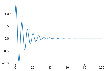
24 t = np.append(np.arange(0,100,0.01),100)
25 theta_euler = euler_theta(t)
26 plt.plot(t,theta_euler)
![]()
1 # the two first order differential equations
2 def f(t,theta1,theta2):
3 return theta2
4
5 def g(t,theta1,theta2):
6 return -0.2*theta2 - (9.8/10)*np.sin(theta1)
7
8 # RK4
9 def rk4_theta(t):
10
11 n = len(t)
12 h = t[1] - t[0]
13
14 theta1 = np.zeros(n)
15 theta1[0] = np.pi/3
16 theta2 = np.zeros(n)
17 theta2[0] = np.pi/4
18
19 for i in range(0,n-1):
20
21 f1 = f(t[i], theta1[i], theta2[i])
22 g1 = g(t[i], theta1[i], theta2[i])
23
24 f2 = f(t[i]+h/2, theta1[i]+h/2*f1, theta2[i]*h/2*g1)
25 g2 = g(t[i]+h/2, theta1[i]+h/2*f1, theta2[i]*h/2*g1)
26
27 f3 = f(t[i]+h/2, theta1[i]+h/2*f2, theta2[i]*h/2*g2)
28 g3 = g(t[i]+h/2, theta1[i]+h/2*f2, theta2[i]*h/2*g2)
29
30 f4 = f(t[i]+h, theta1[i]+h*f3, theta2[i]*h*g3)
31 g4 = g(t[i]+h, theta1[i]+h*f3, theta2[i]*h*g3)
32
33 theta1[i+1] = theta1[i] + h/6*(f1 + 2*f2 + 2*f3 + f4)
34 theta2[i+1] = theta2[i] + h/6*(g1 + 2*g2 + 2*g3 + g4)
35
36 return theta1
37
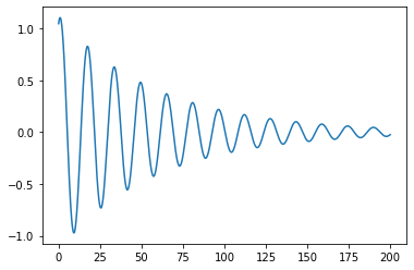
38 t = np.append(np.arange(0,200,0.01),200)
39 theta_rk4 = rk4_theta(t)
40 plt.plot(t,theta_rk4)
![]()
1 # SciPy
2 from scipy import integrate
3
4 def solve(theta,t):
5     return [theta[1], -0.2*theta[1] - (9.8/10)*np.sin(theta[0]) ]
6
7 t = np.append(np.arange(0,100,0.01),100)
8 theta = integrate.odeint(solve, [np.pi/3, np.pi/4], t)
9 plt.plot(t,theta[:,0])
![]()
1 def euler_theta(t):
2
3 n = len(t)
4 h = t[1] - t[0]
5
6 theta1 = np.zeros(n)
7 theta1[0] = np.pi/3
8 theta2 = np.zeros(n)
9 theta2[0] = np.pi/4
10
11 for i in range(0,n-1):
12
13 theta1[i+1] = theta1[i] + h*f(t[i], theta1[i], theta2[i])
14 theta2[i+1] = theta2[i] + h*g(t[i], theta1[i], theta2[i])
15
16 return theta1
17
18 def euler_velocity(t):
19
20 n = len(t)
21 h = t[1] - t[0]
22
23 theta1 = np.zeros(n)
24 theta1[0] = np.pi/3
25 theta2 = np.zeros(n)
26 theta2[0] = np.pi/4
27
28 for i in range(0,n-1):
29
30 theta1[i+1] = theta1[i] + h*f(t[i], theta1[i], theta2[i])
31 theta2[i+1] = theta2[i] + h*g(t[i], theta1[i], theta2[i])
32
33 return theta2
34
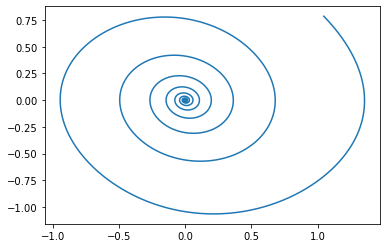
35 t = np.append(np.arange(0,100,0.01),100)
36 theta_euler = euler_theta(t)
37 velocity_euler = euler_velocity(t)
38 plt.plot(theta_euler,velocity_euler)
![]()
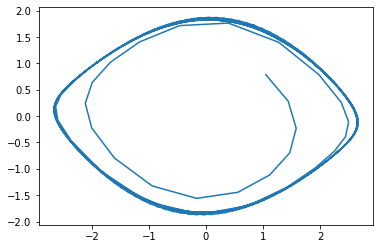
1 t = np.append(np.arange(0,100,0.5),100)
2 theta_euler = euler_theta(t)
3 velocity_euler = euler_velocity(t)
4 plt.plot(theta_euler,velocity_euler)
![]()


 浙公网安备 33010602011771号