1 # import packages
2 import matplotlib.pyplot as plt
3 import numpy as np
4 import time
5 from mpl_toolkits.mplot3d import Axes3D
6 from matplotlib import cm  # cm, colormap, command similar to plt
7 import scipy.integrate as integrate
 1 # initialparameters
 2 # h = 30   # height of the house
 3 # X = np.arange(a,b,10)  # area szie and stepsize
 4 # Y = np.arange(a,b,10)
 5 # X, Y = np.meshgrid(X,Y)
 6 xmin = -4
 7 xmax = 6
 8 ymin = -6
 9 ymax = 4
10 N = 20
11 X = np.linspace(xmin,xmax,N)
12 Y = np.linspace(ymin,ymax,N)
13 X,Y = np.meshgrid(X,Y)
14
15 # Levi function N.13
16 A1 = 1.5
17 x1 = 2.02083
18 y1 = -0.172881
19 sigmax1 = 0.1
20 sigmay1 = 0.35
21 Gaussian1 = A1*np.exp(-1.0*(X-x1)**2/(2*sigmax1))*np.exp(-1.0*(Y-y1)**2/(2*sigmay1))
22
23 A2 = 6.0
24 x2 = 0.8
25 y2 = -2.0
26 sigmax2 = 5.0
27 sigmay2 = 0.7
28 Gaussian2 = A2*np.exp(-1.0*(X-x2)**2/(2*sigmax2))*np.exp(-1.0*(Y-y2)**2/(2*sigmay2))
29 Z = Gaussian1+Gaussian2
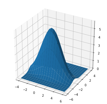
1 fig = plt.figure(figsize=(6,6))
2 ax = fig.add_subplot(111, projection='3d') # projection
3
4 # plot a 3D surface
5 ax.plot_surface(X,Y,Z)
6 plt.savefig('Contour_surface.png',format='png', bbox_inches='tight', dpi=72)
7 plt.show()
8
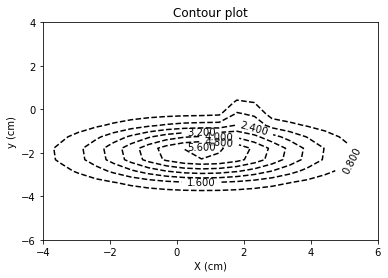
9 plt.figure(2)
10 cp = plt.contour(X, Y, Z, colors='black', linestyles='dashed')
11 plt.clabel(cp, inline=True,
12 fontsize=10)
13 plt.title('Contour plot')
14 plt.xlabel('X (cm)')
15 plt.ylabel('y (cm)')
16 plt.savefig('Contour_line.png',format='png', bbox_inches='tight', dpi=72)
17 plt.show()
![]()
![]()
 1 dx = X[0,1]-X[0,0]
 2 dy = Y[1,0]-Y[0,0]
 3 Integral = Z[:N-1,:N-1].sum()*dx*dy # volume integrate
 4 # print(dx,dy,Integral)
 5
 6 s = np.zeros(N)
 7 for i in range(N):
 8     s[i] = integrate.simps(Z[:,i], dx=dx)  # surface integrate i
 9     Volume_Simpson = integrate.simps(s,dx=dy)  # volume integrate
10 print(Integral, Volume_Simpson)


 浙公网安备 33010602011771号