深度学习--RBM(Restricted Boltzmann Machine)受限玻尔兹曼机-算法--91
1. 原理
参考: https://bacterous.github.io/2018/05/22/Restricted Boltzmann Machine/
受限玻尔兹曼机(Restricted Boltzmann Machine,RBM)是G.Hinton教授的一宝。
Hinton教授是深度学习的开山鼻祖,也正是他在2006年的关于深度信念网络DBN的工作,以及逐层预训练的训练方法,开启了深度学习的序章。其中,DBN中在层间的预训练就采用了RBM算法模型。RBM是一种无向图模型,也是一种神经网络模型。
深度信念网络DBN可以参考:
https://snowkylin.github.io/blogs/DBN.html
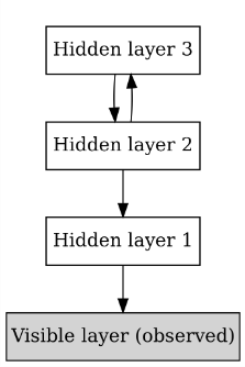
深度信念网络(Deep Belief Networks, DBNs)由Geoffrey Hinton于2006年提出,是一种经典的深度生成式模型,通过将一系列受限玻尔兹曼机(RBM)单元堆叠而进行训练。这一模型在MNIST数据集上的表现超越了当时流行的SVM,从而开启了深度学习在学术界和工业界的浪潮,在深度学习的发展历史中具有重要意义。尽管随着大量表现更好的深度学习算法的出现,深度信念网络已经很少使用,但其理论的优美性、方法的开创性和历史意义的重要性。
回到RBM受限玻尔兹曼机,
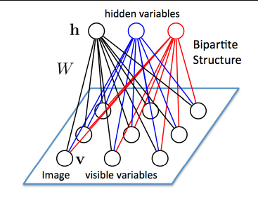
RBM具有两层:可见层(V层),以及隐藏层(H层)。可以看到,两层神经元之间都是全连接的,但是每一层各自的神经元之间并没有连接,也就是说,RBM的图结构是一种二分图(bipartite graph)。
正是这个特点,才叫受限玻尔兹曼机,玻尔兹曼机是允许同一层之间的神经元相连的。RBM其实是一种简化了的BM模型。
还有一个特点,RBM中的神经元都是二值化的,也就是说只有激活和不激活两种状态,也就是0或者1;可见层和隐藏层之间的边的权重可以用W来表示,
W是一个VxH大小的实数矩阵。
算法难点主要就是对W求导,用于梯度下降的更新;但是因为V和H都是二值化的,没有连续的可导函数去计算,实际中采用的sampling的方法来计算,
这里面就可以用比如Gibbs sampling的方法,当然,Hinton提出了对比散度Constractive Divergence CD方法,比Gibbs方法更快,已经成为求解RBM的标准解法。
Restricted Boltzmann Machines(RBM)是一种用于无监督学习的生成型随机神经网络。它们通常用于特征学习、降维和推荐系统等领域。RBM的核心思想是通过学习数据的概率分布来捕捉数据中的潜在结构。
RBM的核心思想是通过学习数据的概率分布来捕捉数据中的潜在结构。
RBM通过调整权重和偏置来学习数据的概率分布。
练过程中,RBM通过正向传播(从可见层到隐藏层)和反向传播(从隐藏层到可见层)来更新权重和偏置。
正向传播:输入数据(可见层)通过权重矩阵传递到隐藏层,隐藏层的神经元根据传递过来的值以一定的概率激活。
反向传播:激活的隐藏层神经元通过相同的权重矩阵传递回可见层,生成新的可见层数据。
通过比较原始输入数据和生成的数据,调整权重和偏置,使得生成的数据尽可能接近原始数据。
应用:
RBM可以用于特征提取,将原始数据转换为更抽象的特征表示。
RBM也可以用于降维,将高维数据映射到低维空间。
RBM还可以用于推荐系统,通过学习用户和物品的潜在特征来预测用户对物品的偏好。
2. 结构
RBM由两层组成:可见层(visible layer)和隐藏层(hidden layer)。
可见层包含输入数据,隐藏层包含从可见层学习到的特征。
层与层之间的神经元是全连接的,但同一层内的神经元之间没有连接。
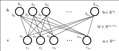
因为RBM隐层和可见层是全连接的,为了描述清楚与容易理解,把每一层的神经元展平即可,
RBM是一个能量模型(Energy based model, EBM),是从物理学能量模型中演变而来;能量模型需要做的事情就是先定义一个合适的能量函数,然后基于这个能量函数得到变量的概率分布,最后基于概率分布去求解一个目标函数(如最大似然)。RBM的过程如下:
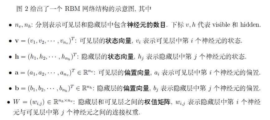
现在变量是(v,h),包括隐层和可见层神经元;参数包括θ=(W,a,b)。能量函数定义:

如果写成向量/矩阵:

3. 代码实现RBM-01
import numpy as np
import tensorflow as tf
from tensorflow.keras.models import Sequential
from tensorflow.keras.layers import Dense
from tensorflow.keras.optimizers import SGD

# 定义RBM类
class RBM:
    def __init__(self, n_visible, n_hidden, epochs=10, batch_size=32, learning_rate=0.1):
        self.n_visible = n_visible
        self.n_hidden = n_hidden
        self.epochs = epochs
        self.batch_size = batch_size
        self.learning_rate = learning_rate
        self.model = self._build_model()

    def _build_model(self):
        model = Sequential()
        model.add(Dense(self.n_hidden, input_dim=self.n_visible, activation='sigmoid'))
        model.add(Dense(self.n_visible, activation='sigmoid'))
        model.compile(optimizer=SGD(learning_rate=self.learning_rate), loss='mean_squared_error')
        return model

    def fit(self, X):
        for epoch in range(self.epochs):
            for i in range(0, len(X), self.batch_size):
                batch = X[i:i + self.batch_size]
                hidden_probs = self.model.predict(batch)
                visible_probs = self.model.predict(hidden_probs)
                self.model.train_on_batch(batch, visible_probs)
            print(f"Epoch {epoch + 1}/{self.epochs} completed")

    def transform(self, X):
        return self.model.predict(X)

# 示例数据
X = np.array([[0, 0, 1, 1], [1, 1, 0, 0], [1, 0, 0, 1], [0, 1, 1, 0]])

# 创建RBM实例
rbm = RBM(n_visible=4, n_hidden=2, epochs=10, batch_size=2, learning_rate=0.1)

# 训练RBM
rbm.fit(X)

# 转换数据
transformed_X = rbm.transform(X)
print("Transformed Data:")
print(transformed_X)
输出:
Transformed Data:
[[0.4760437  0.4885459  0.60684925 0.40946364]
 [0.4366482  0.51952857 0.5729282  0.40083942]
 [0.51250404 0.46508545 0.6172081  0.4312686 ]
 [0.4048287  0.5408431  0.5618714  0.38270262]]
4. 代码实现RBM-02
import tensorflow as tf
import numpy as np
import matplotlib.pyplot as plt
(train_data, _), (test_data, _) = tf.keras.datasets.mnist.load_data()
train_data = train_data / np.float32(255)
train_data = np.reshape(train_data, (train_data.shape[0], 784))

test_data = test_data / np.float32(255)
test_data = np.reshape(test_data, (test_data.shape[0], 784))
#Class that defines the behavior of the RBM
class RBM(object):

    def __init__(self, input_size, output_size, lr=1.0, batchsize=100):
        """
        m: Number of neurons in visible layer
        n: number of neurons in hidden layer
        """
        #Defining the hyperparameters
        self._input_size = input_size #Size of Visible
        self._output_size = output_size #Size of outp
        self.learning_rate = lr #The step used in gradient descent
        self.batchsize = batchsize #The size of how much data will be used for training per sub iteration

        #Initializing weights and biases as matrices full of zeroes
        self.w = tf.zeros([input_size, output_size], np.float32) #Creates and initializes the weights with 0
        self.hb = tf.zeros([output_size], np.float32) #Creates and initializes the hidden biases with 0
        self.vb = tf.zeros([input_size], np.float32) #Creates and initializes the visible biases with 0


    #Forward Pass
    def prob_h_given_v(self, visible, w, hb):
        #Sigmoid
        return tf.nn.sigmoid(tf.matmul(visible, w) + hb)

    #Backward Pass
    def prob_v_given_h(self, hidden, w, vb):
        return tf.nn.sigmoid(tf.matmul(hidden, tf.transpose(w)) + vb)

    #Generate the sample probability
    def sample_prob(self, probs):
        return tf.nn.relu(tf.sign(probs - tf.random.uniform(tf.shape(probs))))

    #Training method for the model
    def train(self, X, epochs=10):

        loss = []
        for epoch in range(epochs):
            #For each step/batch
            for start, end in zip(range(0, len(X), self.batchsize),range(self.batchsize,len(X), self.batchsize)):
                batch = X[start:end]

                #Initialize with sample probabilities

                h0 = self.sample_prob(self.prob_h_given_v(batch, self.w, self.hb))
                v1 = self.sample_prob(self.prob_v_given_h(h0, self.w, self.vb))
                h1 = self.prob_h_given_v(v1, self.w, self.hb)

                #Create the Gradients
                positive_grad = tf.matmul(tf.transpose(batch), h0)
                negative_grad = tf.matmul(tf.transpose(v1), h1)

                #Update learning rates
                self.w = self.w + self.learning_rate *(positive_grad - negative_grad) / tf.dtypes.cast(tf.shape(batch)[0],tf.float32)
                self.vb = self.vb +  self.learning_rate * tf.reduce_mean(batch - v1, 0)
                self.hb = self.hb +  self.learning_rate * tf.reduce_mean(h0 - h1, 0)

            #Find the error rate
            err = tf.reduce_mean(tf.square(batch - v1))
            print ('Epoch: %d' % epoch,'reconstruction error: %f' % err)
            loss.append(err)

        return loss

    #Create expected output for our DBN
    def rbm_output(self, X):
        out = tf.nn.sigmoid(tf.matmul(X, self.w) + self.hb)
        return out

    def rbm_reconstruct(self,X):
        h = tf.nn.sigmoid(tf.matmul(X, self.w) + self.hb)
        reconstruct = tf.nn.sigmoid(tf.matmul(h, tf.transpose(self.w)) + self.vb)
        return reconstruct
input_size = train_data.shape[1]
rbm = RBM(input_size, 200)
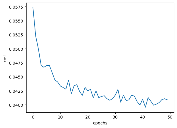
err = rbm.train(train_data, 50)
Epoch: 0 reconstruction error: 0.057316
Epoch: 1 reconstruction error: 0.052252
Epoch: 2 reconstruction error: 0.049920
Epoch: 3 reconstruction error: 0.047002
Epoch: 4 reconstruction error: 0.046681
Epoch: 5 reconstruction error: 0.047001
Epoch: 6 reconstruction error: 0.047006
Epoch: 7 reconstruction error: 0.045737
Epoch: 8 reconstruction error: 0.044407
Epoch: 9 reconstruction error: 0.044064
Epoch: 10 reconstruction error: 0.043346
Epoch: 11 reconstruction error: 0.043070
Epoch: 12 reconstruction error: 0.042784
Epoch: 13 reconstruction error: 0.044382
Epoch: 14 reconstruction error: 0.041971
Epoch: 15 reconstruction error: 0.043392
Epoch: 16 reconstruction error: 0.043581
Epoch: 17 reconstruction error: 0.042389
Epoch: 18 reconstruction error: 0.041673
Epoch: 19 reconstruction error: 0.043095
Epoch: 20 reconstruction error: 0.042499
Epoch: 21 reconstruction error: 0.042730
Epoch: 22 reconstruction error: 0.041233
Epoch: 23 reconstruction error: 0.042468
Epoch: 24 reconstruction error: 0.041262
Epoch: 25 reconstruction error: 0.041479
Epoch: 26 reconstruction error: 0.041599
Epoch: 27 reconstruction error: 0.041076
Epoch: 28 reconstruction error: 0.040802
Epoch: 29 reconstruction error: 0.041052
Epoch: 30 reconstruction error: 0.041701
Epoch: 31 reconstruction error: 0.042723
Epoch: 32 reconstruction error: 0.040449
Epoch: 33 reconstruction error: 0.041692
Epoch: 34 reconstruction error: 0.040725
Epoch: 35 reconstruction error: 0.040880
Epoch: 36 reconstruction error: 0.041719
Epoch: 37 reconstruction error: 0.041507
Epoch: 38 reconstruction error: 0.040551
Epoch: 39 reconstruction error: 0.039942
Epoch: 40 reconstruction error: 0.040974
Epoch: 41 reconstruction error: 0.039551
Epoch: 42 reconstruction error: 0.041289
Epoch: 43 reconstruction error: 0.040623
Epoch: 44 reconstruction error: 0.039917
Epoch: 45 reconstruction error: 0.040104
Epoch: 46 reconstruction error: 0.040372
Epoch: 47 reconstruction error: 0.040910
Epoch: 48 reconstruction error: 0.041071
Epoch: 49 reconstruction error: 0.040880
plt.plot(err)
plt.xlabel('epochs')
plt.ylabel('cost')

out = rbm.rbm_reconstruct(test_data)

# Plotting original and reconstructed images
row, col = 2, 8
idx = np.random.randint(0, 100, row * col // 2)
f, axarr = plt.subplots(row, col, sharex=True, sharey=True, figsize=(20,4))
for fig, row in zip([test_data,out], axarr):
    for i,ax in zip(idx,row):
        ax.imshow(tf.reshape(fig[i],[28, 28]), cmap='Greys_r')
        ax.get_xaxis().set_visible(False)
        ax.get_yaxis().set_visible(False)


 浙公网安备 33010602011771号