深度学习--SOM(Self-Organizing Maps,自组织映射)算法--90
参考链接扩展:
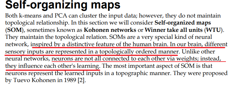
书上看到了关于SOM的介绍,还比较全面:
https://blog.csdn.net/rc15680632552/article/details/123892549
通过距离的计算,确定获胜神经元,winner take all,获胜神经元通过加强自身以及周围临近神经元,而抑制较远的神经元,确保相同的数据(或者类似接近的数据)输入,winner 或者winner 的周围 能再次成为winner ,
读到这一步,深吸一口气,人类社会与这个机制多么接近,一人得道鸡犬升天。名门望族也不是一天两天起来的,贾史王薛,蒋宋孔陈,唉唉唉!
1. 介绍
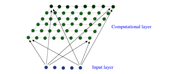
SOM(Self-Organizing Maps,自组织映射)是一种用于数据可视化和降维的神经网络算法。它可以将高维数据映射到低维空间(通常是二维),同时保持数据的拓扑结构。SOM在模式识别、数据挖掘和神经信息处理等领域有广泛应用。
sometimes known as Kohonen networks or Winner take all units (WTU).
注意神经元之间并不会直接相连,神经元只与输入节点相连,
通俗解释:
想象一下,你有一堆形状和颜色各异的玩具,你想把它们分类并摆放在一个二维的架子上,使得相似的玩具放在一起。SOM算法就是帮你完成这个任务的工具。它会自动学习哪些玩具相似,并将它们放在架子上相邻的位置。
2. 工作原理
-
初始化:首先,我们在二维平面上随机初始化一些神经元,每个神经元都有一个权重向量,这个向量的维度与输入数据的维度相同。
-
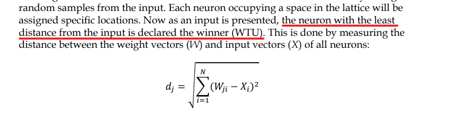
竞争:对于每一个输入数据,计算它与每个神经元权重向量的距离。距离最近的神经元被称为“获胜神经元”或“最佳匹配单元(BMU)”。
![]()
-
合作与适应:获胜神经元及其邻近的神经元会调整它们的权重向量,使其更接近输入数据。这个过程通过学习率和邻域函数来控制。
![]()
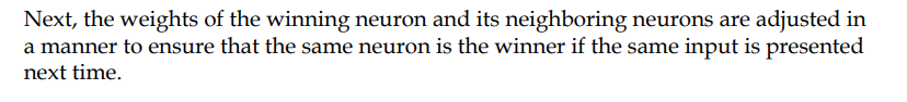
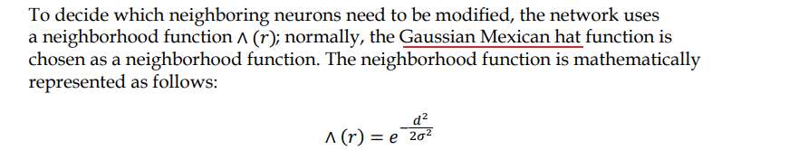
𝜎 is a time-dependent radius of influence of a neuron
d is its distance from the winning neuron
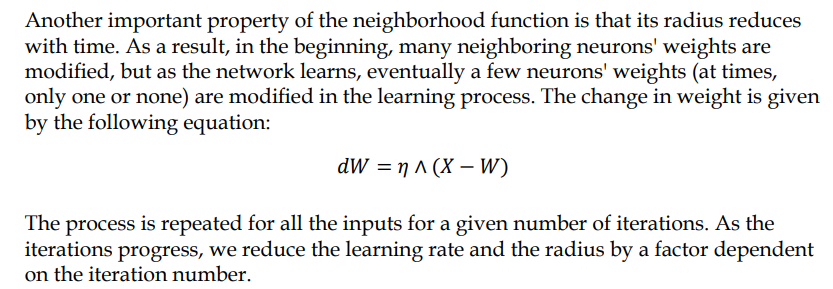
4. 迭代:重复上述步骤,直到神经元的权重向量不再显著变化或达到预定的迭代次数。
墨西哥 帽

权重的更新:

3. 代码
import tensorflow as tf
import numpy as np
import matplotlib.pyplot as plt
# define the winner take all units
class WTU:
    def __init__(self, m, n, dim, num_iterations, eta=0.5, sigma=None):
        """
        m x n: the dimension of 2D lattice in which nuerons are arranged
        dim: Dimension of input training data
        num_iterations: Total number of training iterations
        eta: Learning rate
        sigma: The ratius of neighbourhood function
        """
        self._m = m
        self._n = n
        self._neighbourhood = []
        self._topography = []
        self._num_iterations = int(num_iterations)
        self._learned = False
        self.dim = dim

        self.eta = float(eta)

        if sigma is None:
            sigma = max(m, n) / 2.0  # Constant radius
        else:
            sigma = float(sigma)
        self.sigma = sigma
        print("Net created with dimension:", m , n)

        # wight Matric and the topography of neurons
        self._W = tf.random.normal([m*n, dim], seed=0)
        #print("W:", self._W)
        self._topography = np.array(list(self._nueron_loation(m, n)))
        #print("topography:", self._topography)


    def _nueron_loation(self,m, n):
        for i in range(m):
            for j in range(n):
                yield np.array([i, j])

    def training(self, x, i):
        m = self._m
        n = self._n

        # finding the winner and its location

        # 计算输入向量 x 与权重矩阵 _W 中每个权重向量的欧氏距离。
        d = tf.sqrt(tf.reduce_sum(tf.pow(self._W - tf.stack([x for i in range(m*n)]),2),1))
        # 到距离最小的权重向量,即获胜神经元
        self.WTU_idx = tf.argmin(d, 0)

        # 获取获胜神经元的位置
        # 使用获胜神经元的索引 WTU_idx 从神经元位置矩阵 _topography 中提取获胜神经元的位置

        slice_start = tf.pad(tf.reshape(self.WTU_idx, [1]),np.array([[0,1]]))
        """
        self.WTU_idx 是一个标量,表示获胜神经元的索引
        举例 _topography=[[0,0], [0,1], [0,2],    [1,0,], [1,1], [1,2],     [2,0,], [2,1], [2,2]]
        WTU_idx为其中一个: 0       1       2        3      4     5            6       7     8
        假设 WTU_idx =5
        tf.reshape(self.WTU_idx, [1]) 将这个标量转换为一个形状为 [1] 的张量。-->  [5]
        tf.pad(..., np.array([[0,1]]))  --> [5,0]
        """


        self.WTU_loc = tf.reshape(tf.slice(self._topography, slice_start,[1,2]), [2])
        """
        self._topography 是一个形状为 [m*n, 2] 的张量,其中 m 和 n 是 SOM 网络的维度,每一行表示一个神经元的位置(二维坐标)。
        tf.slice(self._topography, slice_start, [1,2])
        从 self._topography 中提取一个切片。
        slice_start 是开始切片的索引,[1,2] 表示切片的形状。
        这里 slice_start 的第一个元素是获胜神经元的索引,第二个元素是 0(因为我们在上一步中填充了一个 0)
        例如,如果 slice_start 是 [5, 0],
        那么 tf.slice(self._topography, [5, 0], [1, 2]) 将提取 self._topography 中第 5 行的前 2 个元素。
        tf.reshape(..., [2]) 将提取的切片重新整形为一个形状为 [2] 的张量,表示获胜神经元的位置。
        """
        # 总结一下,这两行代码的目的是将获胜神经元的索引 WTU_idx 转换为 _topography 中的位置,并将其存储在 self.WTU_loc 中。


        # Change learning rate and the radius as a function of iterations
        learning_rate = 1 - i/self._num_iterations
        _eta_new = self.eta * learning_rate
        _sigma_new = self.sigma * learning_rate

        # neighbourhood funxtion calculation
        # 计算每个神经元与获胜神经元之间的距离平方  --> (_topography-WTU_loc)**2
        distance_square = tf.reduce_sum(tf.pow(tf.subtract(self._topography, tf.stack([self.WTU_loc for i in range(m*n)])), 2), 1)
        # 使用高斯函数计算邻域函数,距离越远的神经元受到的影响越小
        neighbourhood_func = tf.exp(tf.negative(tf.math.divide(tf.cast(distance_square, tf.float32), tf.pow(_sigma_new, 2))))

        # multipy learning rate with neighbourhood func
        # 将学习率与邻域函数相乘
        eta_into_Gamma = tf.multiply(_eta_new, neighbourhood_func)

        # shape it so that it can be multiplied to calculate dW
        # 将 eta_into_Gamma 扩展到与权重矩阵相同的形状
        weight_multiplier = tf.stack([tf.tile(tf.slice(eta_into_Gamma, np.array([i]), np.array([1])), [self.dim]) for i in range(m*n)])
        """
        1.
        tf.slice(eta_into_Gamma, np.array([i]), np.array([1]))
            tf.slice 用于从张量中提取一个切片。
            eta_into_Gamma 是输入张量。
            np.array([i]) 是起始索引,表示从第 i 个元素开始。
            np.array([1]) 是切片的长度,表示提取一个元素。
        因此,tf.slice(eta_into_Gamma, np.array([i]), np.array([1])) 提取 eta_into_Gamma 的第 i 个元素。

        2.tf.tile(..., [self.dim])
        tf.tile 用于将张量沿着指定维度重复。
            [self.dim] 表示将提取的单个元素重复 self.dim 次,形成一个长度为 self.dim 的向量。

        3.列表推导式 [... for i in range(m*n)]:
        这个列表推导式遍历 i 从 0 到 m*n-1。
        对于每个 i,执行前面的操作,提取 eta_into_Gamma 的第 i 个元素并将其扩展为长度为 self.dim 的向量。

        4. tf.stack(...):
        tf.stack 用于将一个列表中的张量堆叠在一起,形成一个新的张量。
        这里将所有扩展后的向量堆叠在一起,形成一个新的张量 weight_multiplier。

        总结一下,这行代码的作用是:
        从 eta_into_Gamma 中提取每个元素。
        将每个元素扩展为一个长度为 self.dim 的向量。
        将所有这些向量堆叠在一起,形成一个新的张量 eight_multiplier。

        """

        # 计算权重更新量 delta_W=eta*h*(x-m)
        delta_W = tf.multiply(weight_multiplier, tf.subtract(tf.stack([x for i in range(m*n)]), self._W))
        new_W = self._W + delta_W
        self._W = new_W


    def fit(self, X):
        for i in range(self._num_iterations):
            for x in X:
                self.training(x, i)
        # restore the centroid grid for easy retrival
        centroid_grid = [[] for i in range(self._m)]

        self._Wts = list(self._W)
        self._locations = list(self._topography)

        for i, loc in enumerate(self._topography):
            centroid_grid[loc[0]].append(self._Wts[i])
        self._centroid_grid = centroid_grid
        self._learned = True
        print("fit finish !")

    def winner(self, x):
        return self.WTU_idx, self.WTU_loc   # 在_topography中的索引号, 二维坐标

    def get_centroids(self):
        if not self._learned:
            raise ValueError("SOM not train yet")
        return self._centroid_grid
    def map_vects(self, X):
        """
        遍历输入向量 X 中的每一个向量。
        找到与每个输入向量最接近的权重向量。
        将最接近的权重向量对应的 SOM 节点位置添加到结果列表中。
        """
        if not self._learned:
            raise ValueError("SOM not train yet")
        to_return = []
        for vect in X:
            min_index = min([i for i in range(len(self._Wts))], key=lambda x: np.linalg.norm(vect - self._Wts[x]))
            to_return.append(self._locations[min_index])
        """
        使用列表推导式生成一个包含所有权重向量索引的列表 [i for i in range(len(self._Wts))]。
        使用 min 函数找到与当前向量 vect 最接近的权重向量索引 min_index。
        key=lambda x: np.linalg.norm(vect - self._Wts[x]) 是一个关键函数,
        用于计算向量 vect 和权重向量 self._Wts[x] 之间的欧几里得距离(使用 np.linalg.norm 函数)。
        """
        return to_return
def normalize(df):
    result = df.copy()

    for feature_name in df.columns:
        max_value = df[feature_name].max()
        min_value = df[feature_name].min()
        result[feature_name] = (df[feature_name]-min_value)/(max_value - min_value)
    return result.astype(np.float32)  # 注意转换成float32
import pandas as pd
df = pd.read_csv("colors.csv")
data = normalize(df[["R", "G", "B"]]).values
name = df["Color-Name"].values
n_dim = len(df.columns) - 1
colors = data
color_names = name
som = WTU(20, 20, n_dim, 100, sigma=10.0)
som.fit(colors)
Net created with dimension: 20 20
image_grid = som.get_centroids()
mapped = som.map_vects(colors)
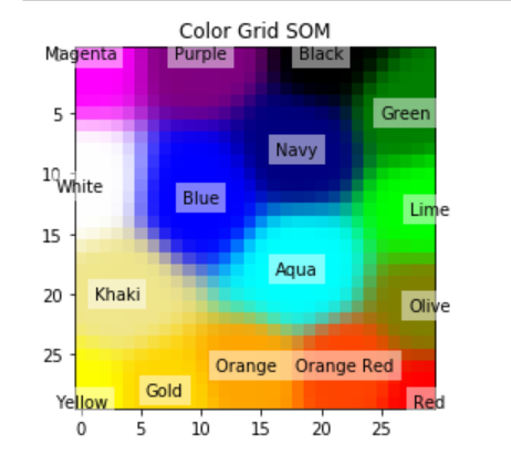
# plot
plt.imshow(image_grid)
plt.title("Color Grid SOM")
for i, m in enumerate(mapped):
plt.text(m[1], m[0], color_names[i], ha='center', va='center', bbox=dict(facecolor='white', alpha=0.5, lw=0))

 浙公网安备 33010602011771号