深度学习-nlp-循环神经网络RNN之LSTM--71
强烈建议阅读:http://colah.github.io/posts/2015-08-Understanding-LSTMs/
Long range temporal dependency(长程时间依赖)指的是在时间序列数据中,当前时间步所依赖的信息与之前的时间步之间的距离较远,甚至可能是整个序列。这种依赖关系在很多任务中都非常重要,例如自然语言处理中的句子理解和生成、语音识别中的语音转文字、股票价格预测等。解决长程时间依赖问题的方法包括使用循环神经网络(RNN)、长短时记忆网络(LSTM)和门控循环单元(GRU)等模型。这些模型能够捕捉到时间序列数据中的长程依赖关系,从而提高模型的预测准确性。
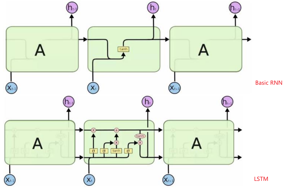
1. 复习Basic RNN
先复习下Basic RNN
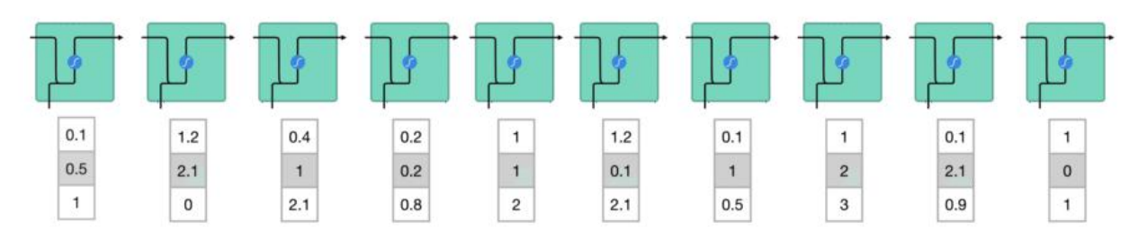
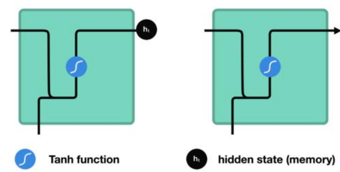
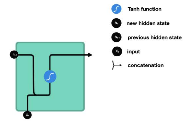
S_t = f(UX_t+WS_t-1)
代码实现:matmul([X_t, S_t-1],transpose([U, W]))
在用tanh激活函数激活
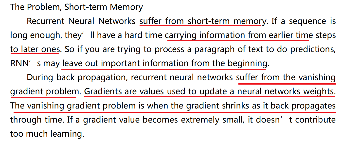
存在的问题:
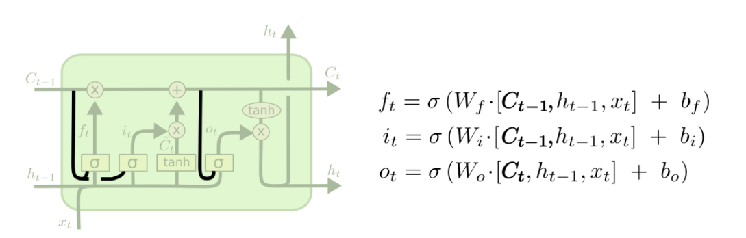
2. LSTM 长短期记忆 网络结构
long short term memory
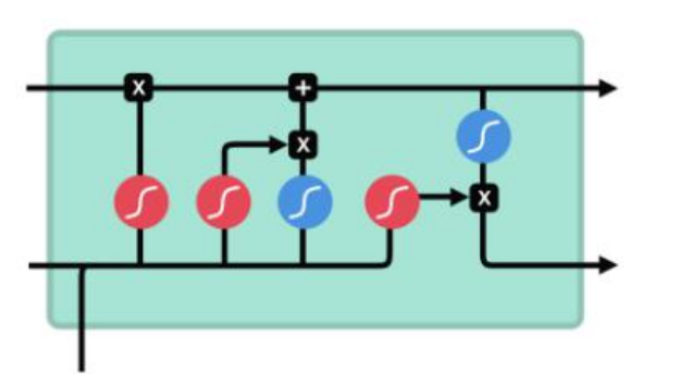

Forget gate,input gate, output gate
To review, the Forget gate decides what is relevant to keep from prior steps. The input gate decides what information is relevant to add from the current step. The output gate determines what the next hidden state should be.
LSTM 两条平行线传递
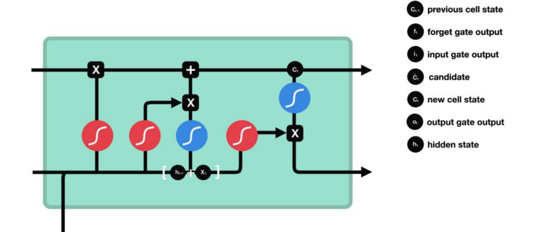
6个公式:
foeget gate
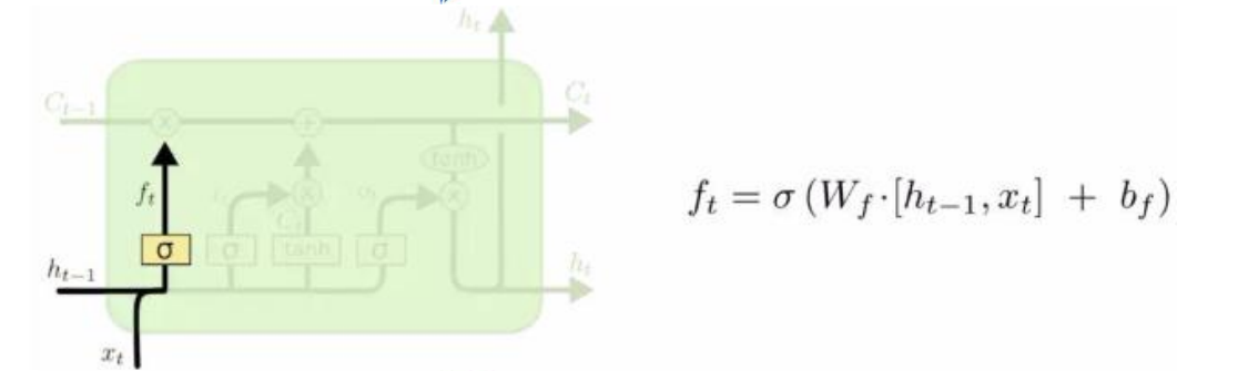
(Wf bf)是需要学习的
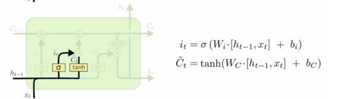
(Wi bi),(Wc bc)是需要学的
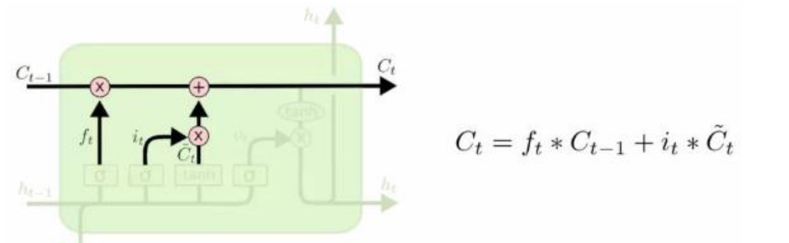
没有需要学的
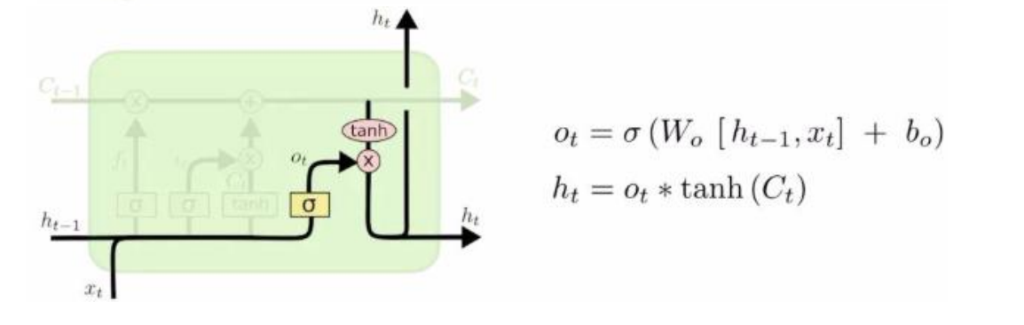
(Wo bo)是需要学的
仔细看这张图
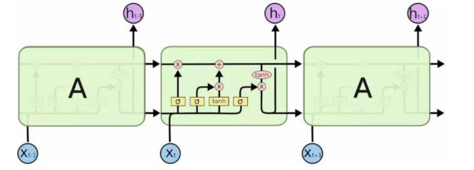
正方形的黄色框 是有需要学习的矩阵 [h_t-1, X_t]会 分别于这4个矩阵相乘
3. RNN实现手写数字识别
Basic RNN
def RNN(X, weights, biases):
    rnn_cell = tf.nn.rnn_cell.BasicRNNCell(n_hidden_units)
    _init_state = rnn_cell.zero_state(batch_size, dtype=tf.float32)
    outputs, last_state = tf.nn.dynamic_rnn(rnn_cell, X, initial_state=_init_state, time_major=False)
    results = tf.matmul(last_state, weights['out'])  + biases['out']

    return results
LSTM RNN
def RNN(X, weights, biases):
    lstm_cell = tf.nn.rnn_cell.BasicLSTMCell(n_hidden_units, forget_bias=1.0, state_is_tuple=True)
    _init_state = lstm_cell.zero_state(batch_size, dtype=tf.float32)
    outputs, last_states = tf.nn.dynamic_rnn(lstm_cell, X, initial_state=_init_state, time_major=False)  # time_major 输入X n_steps时间是在哪个维度
    results = tf.matmul(last_states[1], weights['out']) + biases['out']
    return results
双向LSTM
def RNN(X, weights, biases):
    # lstm 模型正方向传播的 RNN
    lstm_fw_cell = tf.nn.rnn_cell.BasicLSTMCell(n_hidden_units,
                                                forget_bias=1.0)
    initial_state_fw = lstm_fw_cell.zero_state(batch_size, dtype=tf.float32)

    # 反方向传播的 RNN
    lstm_bw_cell = tf.nn.rnn_cell.BasicLSTMCell(n_hidden_units,
                                                forget_bias=1.0)
    initial_state_bw = lstm_bw_cell.zero_state(batch_size, dtype=tf.float32)

    outputs, output_states = tf.nn.bidirectional_dynamic_rnn(
        lstm_fw_cell, lstm_bw_cell, X,
        initial_state_bw=initial_state_bw,
        initial_state_fw=initial_state_fw)
    """
    print(outputs[0].shape) #(40, 10, 100),前向RNN
    print(outputs[1].shape) #(40, 10, 200),后向RNN
    print(output_states[0].c.shape) #(10, 100)前向RNN的c状态
    print(output_states[0].h.shape) #(10, 100)前向RNN的h状态
    print(output_states[1].c.shape) #(10, 200)后向向RNN的c状态
    print(output_states[1].h.shape) #(10, 200)后向向RNN的h状态

    """
    results = tf.matmul(output_states[1].h, weights['out']) + biases['out']

    return results
完整代码:
import tensorflow as tf
from tensorflow.examples.tutorials.mnist import input_data
# 读取mnist数据集,one_hot=True将y列编码为维度10分类的0,1编码
mnist = input_data.read_data_sets('MNIST_data_bak', one_hot=True)
# 打印输出训练集的形状(55000, 784)
print(mnist.train.images.shape)
# 超参数
lr = 0.001
training_iters = 100000
batch_size = 128
n_inputs = 28
n_steps = 28 # RNN 序列的长度 时刻数
n_hidden_units = 128
n_classes = 10
# 图输入
x = tf.placeholder(tf.float32, [None, n_steps, n_inputs]) # 每张图片是28*28 把图片分解层 一行一行传给RNN
y = tf.placeholder(tf.float32, [None, n_classes])
# 定义权重
weights = {
"out": tf.Variable(tf.random_normal([n_hidden_units, n_classes]))
}
biases = {
"out": tf.Variable(tf.constant(0.1, shape=[n_classes, ]))
}
def RNN(X, weights, biases):
# lstm_cell = tf.nn.rnn_cell.BasicLSTMCell(n_hidden_units, forget_bias=1.0, state_is_tuple=True)
# _init_state = lstm_cell.zero_state(batch_size, dtype=tf.float32)
# outputs, last_states = tf.nn.dynamic_rnn(lstm_cell, X, initial_state=_init_state, time_major=False) # time_major 输入X n_steps时间是在哪个维度
# results = tf.matmul(last_states[1], weights['out']) + biases['out']
rnn_cell = tf.nn.rnn_cell.BasicRNNCell(n_hidden_units)
_init_state = rnn_cell.zero_state(batch_size, dtype=tf.float32)
outputs, last_state = tf.nn.dynamic_rnn(rnn_cell, X, initial_state=_init_state, time_major=False)
results = tf.matmul(last_state, weights['out']) + biases['out']
return results
pred = RNN(x, weights, biases)
cost = tf.reduce_mean(tf.nn.softmax_cross_entropy_with_logits(logits=pred, labels=y))
train_op = tf.train.AdamOptimizer(lr).minimize(cost)
correct_pred = tf.equal(tf.argmax(pred, 1), tf.argmax(y, 1))
accuracy = tf.reduce_mean(tf.cast(correct_pred, tf.float32))
init = tf.global_variables_initializer()
with tf.Session() as sess:
sess.run(init)
step = 0
while step * batch_size < training_iters:
batch_xs, batch_ys = mnist.train.next_batch(batch_size)
batch_xs = batch_xs.reshape([batch_size, n_steps, n_inputs])
test_batch_xs, test_batch_ys = mnist.test.next_batch(batch_size)
test_batch_xs = test_batch_xs.reshape([batch_size, n_steps, n_inputs])
_, = sess.run([train_op], feed_dict={
x: batch_xs,
y: batch_ys
})
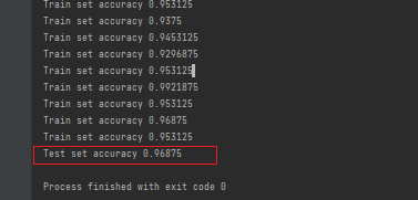
if step % 20 == 0:
print("Train set accuracy %s" % sess.run(accuracy, feed_dict={
x: test_batch_xs,
y: test_batch_ys
}))
step += 1
test_xs, test_ys = mnist.test.next_batch(128)
test_xs = test_xs.reshape([-1, n_steps, n_inputs])
print("Test set accuracy %s" % sess.run(accuracy, feed_dict={
x: test_xs,
y: test_ys
}))
5. LSTM变形
peephole connection 瞭望孔
This means that we let the gate layers look at the cell state.
三个gate可以瞭望记忆细胞里面都有什么。
形象的比喻:潜水艇里面的潜望镜 伸出一根管子出来瞭望
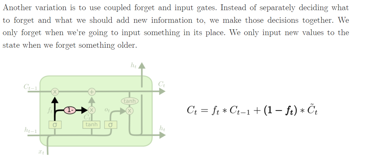
forget与add同时进行
Gated Recurrent Unit, GRU
参考链接:http://arxiv.org/pdf/1406.1078v3.pdf
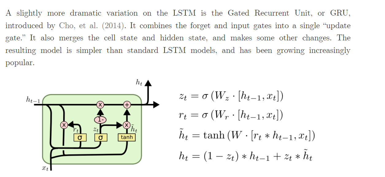
GRU没有记忆cell 认为h_t里面已经包含很多
combines the forget and input gates into a single “update gate”
Hidden Unit that Adaptively Remembersand Forgets。