机器学习-线性回归-逻辑回归-08

目录

• • 1. sigmoid函数
  • 2. 伯努利分布（0-1分布）
  • 3. 广义线性回归
  • 4. 逻辑回归 损失函数的推导
  • 5. 损失函数求导
• 
  • 6. 代码并绘图

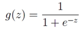
1. sigmoid函数

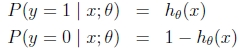
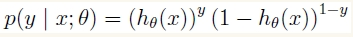
逻辑回归 logitstic regression 本质是二分类
sigmoid函数 是将 （-无穷， +无穷）区间上的y 映射到 （0， 1） 之间的 S型曲线

绘图

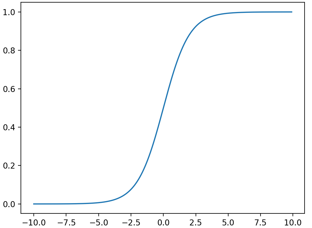
import numpy
import math
import matplotlib.pyplot as plt


def sigmoid(x):
    a = []
    for item in x:
        a.append(1.0 / (1.0 + math.exp(-item)))
    return a

x = numpy.arange(-10, 10, 0.1)
y = sigmoid(x)

plt.plot(x, y)

plt.show()

singmoid 的作用
逻辑回归就是在多元线性回归基础上把结果缩放到0到1之间

2. 伯努利分布（0-1分布）

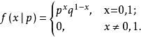
如果随机变量X只有0，1两个值，正样本1 的发生概率为p 则 负样本 的概率为1-p

则称随机变量X服从参数为p的伯努利分布（0-1分布）

q=1-p，则X的概率函数可写

3. 广义线性回归

预测某个随机变量y，y 是某些特征(feature)x的函数。为了推导广义线性模式，我们必须做出如下三个假设

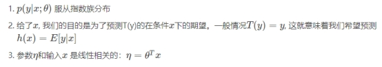
什么是指数族分布
指数族分布（The exponential family distribution)
指数族分布有：高斯分布、二项分布、伯努利分布、多项分布、泊松分布、指数分布、beta分布、拉普拉斯分布、gamma分布

如果应变量y服从某个指数族分布，那么我们就可以用广义线性回归来建模

解释：
η 是 自然参数（natural parameter，also called thecanonical parameter）。
T(y) 是充分统计量 （sufficient statistic） ，一般情况下就是y。
a(η) 是 对数部分函数（log partition function），这部分确保Y的分布p(y:η) 计算的结果加起来（连续函数是积分）等于1。

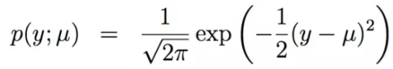
伯努利分布：

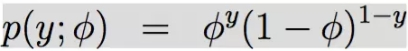
改写成：

由此可知：

线性回归也属于指数族分布的一种：
高斯分布：

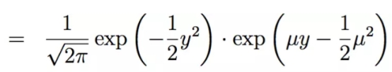
这里面的μ就是指数族分布中的η，所以多元线性回归的形式就是

4. 逻辑回归 损失函数的推导

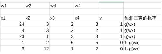
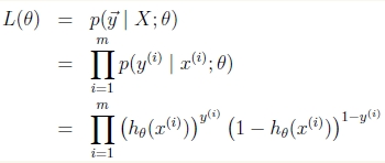
这里我们依然会用到最大似然估计思想，根据若干已知的X,y（训练集）
找到一组W使得X作为已知条件下y发生的概率最大。
样本：

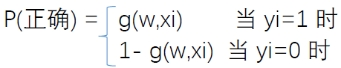
符号重写：

样本相互独立，那么似然函数表达式为

取log 之后：

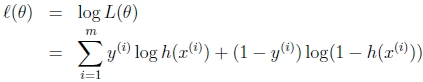
最终损失函数就是上面公式加负号的形式：

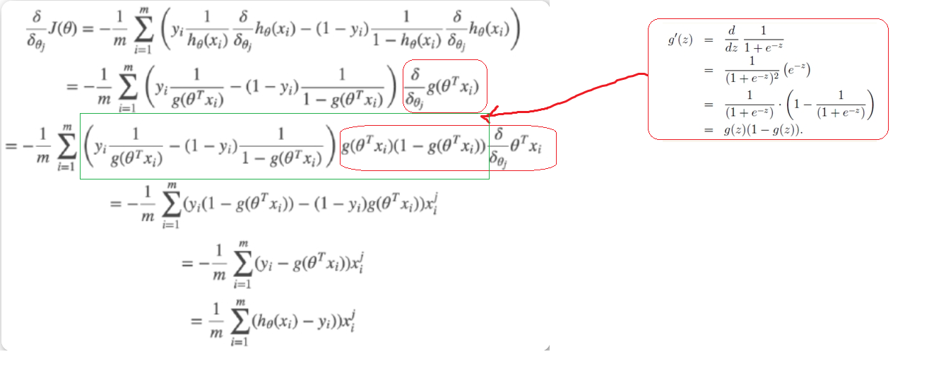
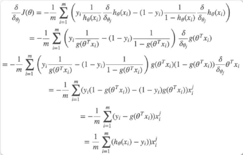
5. 损失函数求导

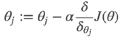
梯度下降法：

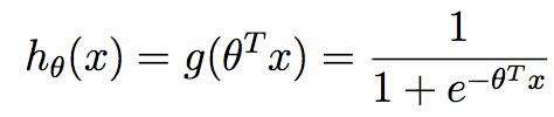
逻辑回归的映射函数

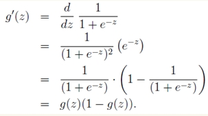
求导：

梯度下降法计算：
逻辑回归：

线性回归：

比较

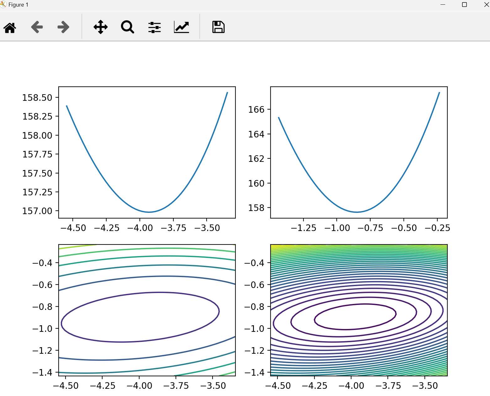
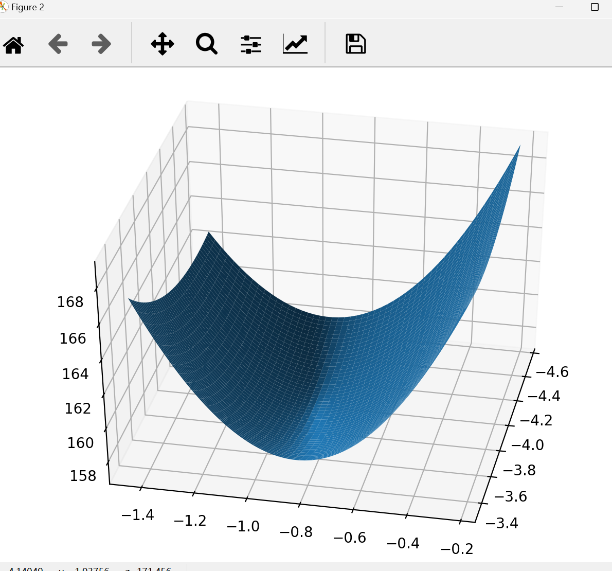
6. 代码并绘图

from sklearn.datasets import load_breast_cancer
from sklearn.linear_model import LogisticRegression
import numpy as np
import matplotlib.pyplot as plt
from mpl_toolkits.mplot3d import Axes3D
from sklearn.preprocessing import scale  # 做样本的归一化处理

data = load_breast_cancer()
# print(data["data"])
# print(data["target"])
X = scale(data['data'][:, :2])  # 取前两个维度
y = data['target']
lr = LogisticRegression(fit_intercept=False)

lr.fit(X, y)

theta1 = lr.coef_[0, 0]
theta2 = lr.coef_[0, 1]

print(theta1, theta1)


# 在已知 theta1 theta2的情况下 根据传进来的数据X 计算y_predict

def p_theta_function(features, w1, w2):
    z = w1 * features[0] + w2 * features[1]
    return 1 / (1 + np.exp(-z))


# 样本 X,y计算损失

def loss_func(sample_features, sample_labels, w1, w2):
    result = 0
    # 遍历数据集中的每一条样本，并且计算每条样本的损失，加到result身上得到整体的数据集损失
    for feature, label in zip(sample_features, sample_labels):  # 一条样本
        p_result = p_theta_function(feature, w1, w2)
        loss_result = -1 * label * np.log(p_result) - (1 - label) * np.log(1 - p_result)
        result += loss_result
    return result


theta1_space = np.linspace(theta1 - 1.0, theta1 + 0.2, 50)
theta2_space = np.linspace(theta2 - 0.6, theta2 + 0.6, 50)

result1_ = np.array([loss_func(X, y, i, theta2) for i in theta1_space])  # 固定theta2不变
result2_ = np.array([loss_func(X, y, theta1, i) for i in theta2_space])

fig1 = plt.figure(figsize=(8, 6))
plt.subplot(2, 2, 1)
plt.plot(theta1_space, result1_)  # theta1 维度 loss的曲线

plt.subplot(2, 2, 2)
plt.plot(theta2_space, result2_)  # theta2 维度 loss的曲线



plt.subplot(2, 2, 3)
theta1_grid, theta2_grid = np.meshgrid(theta1_space, theta2_space)
loss_grid = loss_func(X, y, theta1_grid, theta2_grid)
plt.contour(theta1_grid, theta2_grid, loss_grid)


plt.subplot(2, 2, 4)
plt.contour(theta1_grid, theta2_grid, loss_grid, 30)
fig2 = plt.figure()
ax = Axes3D(fig2)
ax.plot_surface(theta1_grid, theta2_grid, loss_grid)



plt.show()