使用Pytorch构建LSTM网络实现对时间序列的预测

使用Python构建LSTM网络实现对时间序列的预测

1. LSTM网络神经元结构

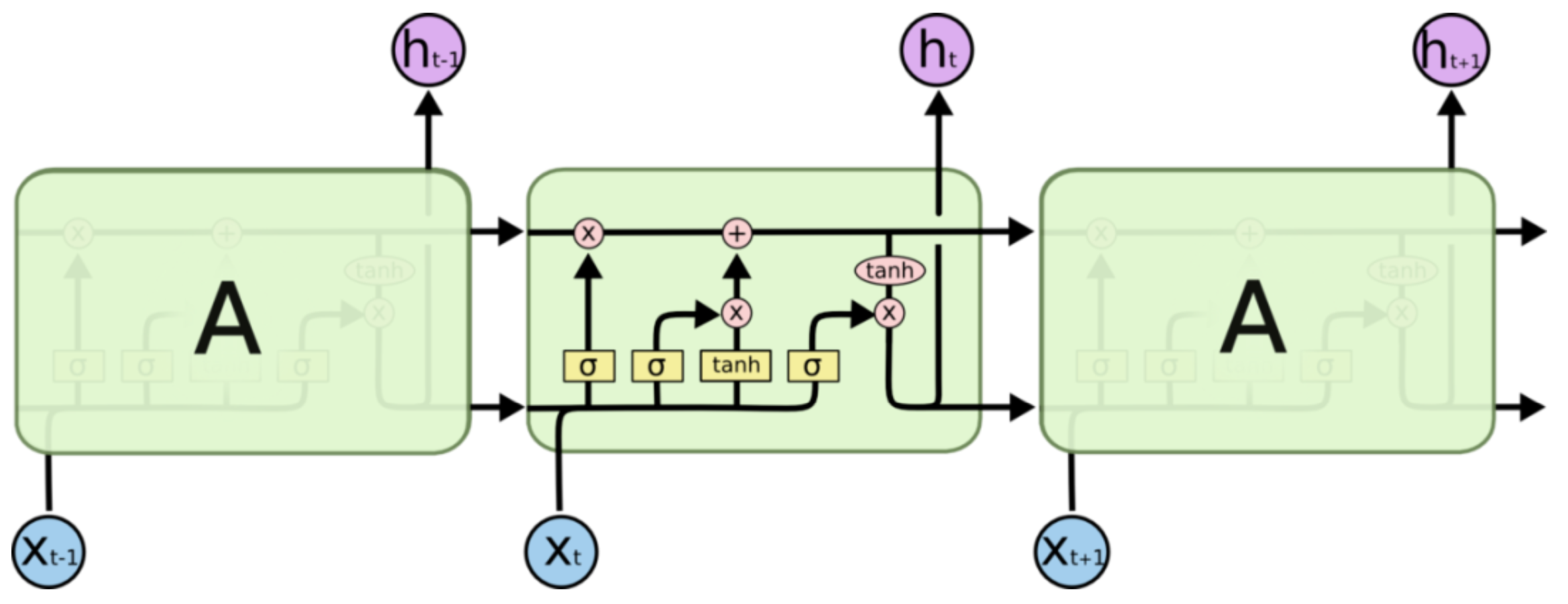
LSTM网络 神经元结构示意图

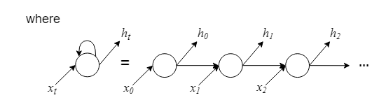
  在任一时刻 $t$，LSTM网络神经元接收该时刻输入信息 $x_t$，输出此时刻的隐藏状态 $h_t$，而 $h_t$ 不仅取决于 $x_t$，还受到 $t-1$ 时刻细胞状态 (cell state) $c_{t-1}$ 和隐藏状态 (hidden state) $h_{t-1}$ 的影响；图中水平贯穿神经元内部的上下两条传送带则分别表示细胞状态及隐藏状态各自从上一时刻传递至下一时刻。

  观察神经元内部结构，黄色方框从左至右可分别看作：

• 遗忘门 (forget gate)：$f_t=\sigma (W_f·[x_t,h_{t-1}]+b_f)$，表示对信息的记忆程度；

• 输入门 (input gate)：$i_t=\sigma (W_i·[x_t,h_{t-1}]+b_i)$，表示对信息的输入强度；

• 状态门 (cell gate)：$g_t=\tanh (W_g·[x_t,h_{t-1}]+b_g)$，表示对输入信息的处理；

• 输出门 (output gate)：$o_t=\sigma (W_o·[x_t,h_{t-1}]+b_o)$，表示对信息的输出强度；

其中， $[x_t,h_{t-1}]$ 表示两向量的并列 (concatenate) 向量，$h_{t-1}$ 表示神经元 $t-1$ 时刻的隐藏状态，$\sigma$ 为 sigmoid 函数。

  在此基础上可更新神经元 $t$ 时刻的细胞状态 $c_t$ 与隐藏状态 $h_t$ 如下：

• $c_t=f_t\odot c_{t-1}+i_t\odot g_t$，即细胞状态 $=$ 经过遗忘后的旧细胞状态 $+$ 神经元处理后的新信息；

• $h_t=o_t\odot \tanh (c_t)$，即隐藏状态 $=$ 输出强度 $\times$ tanh处理后的细胞状态；

其中 $\odot$ 表示哈达玛积 (Hadamard product)，即向量对应元素相乘。

2. 多层LSTM网络

  除去神经元内部结构的特殊性，LSTM 神经网络也分为输入层、隐（藏）层与输出层，输入层、输出层分别对应神经网络模型的输入向量 $X^t=(X_1^t,X_2^t,\dots ,X_D^t)$ 与输出向量 $\widetilde{Y^t}$，神经元个数一般与输入、输出向量的维数一致；同层神经元之间无连接，各隐层神经元接收前一层神经元的输出信号，并输出下一层神经元的接收信号。

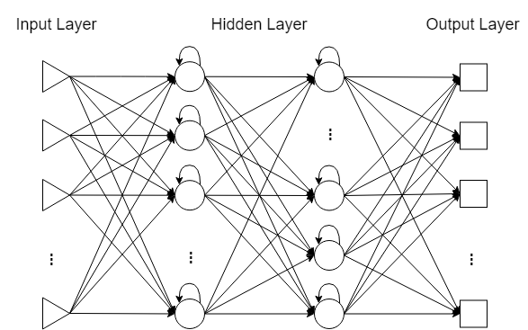
多层LSTM网络结构示意图

• 单层 LSTM 网络:
  隐层神经元的输入信号 $x_t$ 即为 $X^t$；
• 多层 LSTM 网络：
  第 1 层隐层神经元的输入信号 $x_t^{(1)}=X^t$，
  第 $l$ 层 $(l\ge 2)$ 神经元的输入信号 $x_t^{(l)}={\delta }_t^{(l-1)}·h_t^{(l-1)}$，其中 ${\delta }_t^{(l-1)}$ 服从取 0 概率为 dropout 的伯努利分布，dropout 自行指定。

  对于输入向量 $X^t$ 与目标输出向量 $Y^t$，LSTM 神经网络模型总概如下：
训练目标：$par{a}^{\ast }=\underset{paras}{argmin}{\Vert \widetilde{Y^t}-Y^t\Vert }_2$，
训练参数：$paras=\{W_f,b_f;W_i,b_i;W_g,b_g;W_o,b_o\}$，

训练方法：反向传播（本文训练方法），模拟退火法等

[========]

3. 构建 LSTM 网络

声明数据：

• 已知数据 $\mathbf{X}=\{X^1,\dots ,X^m\}$，其中 $X^t=(X_1^t,X_2^t,\dots ,X_D^t),t=1,2,\dots ,m$；
• 预测目标向量 $Y^m=(y^m,y^{m+1},\dots ,y^{m+L-1})=(X_s^m,X_s^{m+1},\dots ,X_s^{m+L-1})$；
  也就是说， 输入数据维度为 $D$，时间点个数为 $m$，预测步长为 $L-1.$

声明 LSTM 网络：

• 输入数据维度 $input\mathrm{\_}size=D$, 隐层神经元个数 (隐层状态 $h_t$ 特征数) $hidden\mathrm{\_}size=n$, 隐层数为 $num\mathrm{\_}layers=l$

import torch
import nn from torch
myLSTM = nn.LSTM(input_size, hidden_size, num_layers)

    LSTM 网络其他参数：

• bias : If False , then the layer does not use bias weights $b_{ih}$ and $b_{hh}$^[1]. Default: True
• batch_first : If True , then the input and output tensors are provided as $(batch\mathrm{\_}size,m,D)$ instead of $(m,batch\mathrm{\_}size,D)$.^[2] Note that this does not apply to hidden or cell states. Default: False.
• dropout : If non-zero , introduces a Dropout layer on the outputs of each LSTM layer except the last layer, with dropout probability equal to dropout. Default: 0
• bidirectional : If True , becomes a bidirectional LSTM (denote $bid=2$). Default: False (denote $bid=1$).
• proj_size : If > 0 , will use LSTM with projections (投影) of corresponding size (denote $H_{out}=pro{j}_{s}ize$). Default: 0 (denote $H_{out}=n$). 换句话说，proj_size 表现了细胞状态与隐藏状态的维数是否一致.

声明 LSTM 网络的输入与输出：

• 网络输入与输出均为张量 (tensor)
• 网络输入：input，($h_0,c_0$)；网络输出: output, ($h_m,c_m$)
• 指导手册上提出了 unbatched inputs 和 outputs 的情况，但在实际操作中，会提示 inputs 必须是 3 维的 (这里可能是笔者的操作有问题，欢迎大家来交流！)

output, (hn, cn) = myLSTM(input, (h0, c0))

	input	$h_0$	$c_0$
unbatched	$(m,D)$	$(bid\times l,H_{out})$	$(bid\times l,n)$
batch_first=True	$(batch\mathrm{\_}size,m,D)$	$(bid\times l,batch\mathrm{\_}size,H_{out})$	$(bid\times l,batch\mathrm{\_}size,n)$
batch_first=False	$(m,batch\mathrm{\_}size,D)$
description	$D$ 维，$m$ 个时间点	初始时刻的隐藏状态 Default：$\overrightarrow{0}$	初始时刻的细胞状态 Default：$\overrightarrow{0}$

	output	$h_m$	$c_m$
unbatched	$(m,bid\times H_{out})$	$(bid\times l,H_{out})$	$(bid\times l,n)$
batch_first=True	$(batch\mathrm{\_}size,m,bid\times H_{out})$	$(bid\times l,batch\mathrm{\_}size,H_{out})$	$(bid\times l,batch\mathrm{\_}size,n)$
batch_first=False	$(m,batch\mathrm{\_}size,bid\times H_{out})$
description	各个时刻 $t$ 最后一层节点的隐藏状态	最终时刻 全部节点的隐藏状态	最终时刻 全部节点的细胞状态
注：对于双向 LSTM 网络，$h_m$ 包含最终时刻的前馈隐藏状态和反馈隐藏状态，而 output 的最后一个元素则是最后一层 节点*最终时刻*的前馈隐藏状态和*初始时刻*的反馈隐藏状态，当 batch_first=False 时可直接分为$(m,batch\mathrm{\_}size,2,H_{out})$.

构建 LSTM 网络结构：

输入数据维度 $input\mathrm{\_}size=D$
隐层神经元个数 (隐层状态 $h_t$ 特征数) $hidden\mathrm{\_}size=n$
隐层数为 $num\mathrm{\_}layers=l$
传播方向为 单向
注：所有 weights 和 bias 的初始值服从均匀分布$\mathcal{U}(-\sqrt{k},\sqrt{k})$，其中 $k=\frac{1}{n}$；
   整个过程可以选择在 GPU 上进行来提高运算速度，此时需要将模型所有的输入向量都转到 GPU 上，具体使用 .to(device) 语句

device = torch.device("cuda:0" if torch.cuda.is_available() else "cpu")
 
class myLSTM(nn.Module):
	def __init__(self, input_size, output_size, hidden_size, num_layers):
		super(myLSTM, self).__init__()
		self.LSTM = nn.LSTM(input_size, hidden_size, num_layers)  # LSTM
		self.reg = nn.Linear(hidden_size, output_size) # regression, 也就是隐藏层到输出层的线性全连接层
 
	def forward(self, x):
		# 在这里，可以指定 (h0, c0)，要记得.to(device)
		# 如果不指定则默认为 0 向量
		x = x.to(device)
		output = self.LSTM(x)[0]  # output, (hm, cm) = self.LSTM(x)
		# output = self.LSTM(x, (h0, c0))[0]
		# seq_len是输入数据的时间点个数
		seq_len, batch_size, hidden_size = output.shape # for default batch_first=False
		# seq_len, hidden_size = output.shape # for unbatched input
		output = output[-1,:,:] #只取最终时刻最后一层节点的隐藏状态做回归，也可以通过hm取
		output = self.reg(output)
		return output

4. 训练 LSTM 网络及预测

# 声明已知数据，可预先进行预处理
train_x # D*(m-L+1)，因为之后时刻的 X^t 对应的 y^t 不完全已知，不同的预测任务可能会有所不同
train_y = train_x[s, :]
train_x = train_x.to(device)
train_y = train_y.to(device)
# 加载模型
net = myLSTM(input_size=D, output_size=L, hidden_size=n, num_layers=l).to(device) # 定义模型
loss = nn.MSELoss().to(device)                                                    #定义损失函数
optimizer = torch.optim.Adam(net.parameters(), lr=1e-2)                           #定义优化器
 
# 开始训练
for i in range(100):          # 迭代次数
	output = net(train_x)     # 向前传播
	Loss = loss(out, train_y) # 计算损失
	optimizer.zero_grad()     # 梯度清零
	Loss.backward()           # 反向传播
	optimizer.step()          # 梯度更新
	if i % 10 == 0:
		print('Epoch: {:4}, Loss: {:.5f}'.format(i, Loss.item()))
 
# 验证 LSTM 网络
test_x # D*m，为全部时刻的数据
pred_y = net(test_x)[0]
pred_y = pred_y[-1,:].item() # 简单预测最终时刻 X^m 对应的目标变量 y^m

5. 总结

5.1 功能总结

5.1 如何理解 batch？

5.2 pad_sequence 的作用？

---

1. $b_{ih}$ 指输入层与隐藏层间的 bias 向量，$b_{hh} 指隐藏层之间的 bias 向量， 也就是 第1部分 中出现的 $\{b_f,b_i,b_g,b_o\}$. ↩︎

2. If inputs are unbatched, then this argument is ignored and the input tensor is $(m,D)$ ↩︎