学习笔记 | Kalman Filter

 

Kalman Filter

Overview:

Steps:

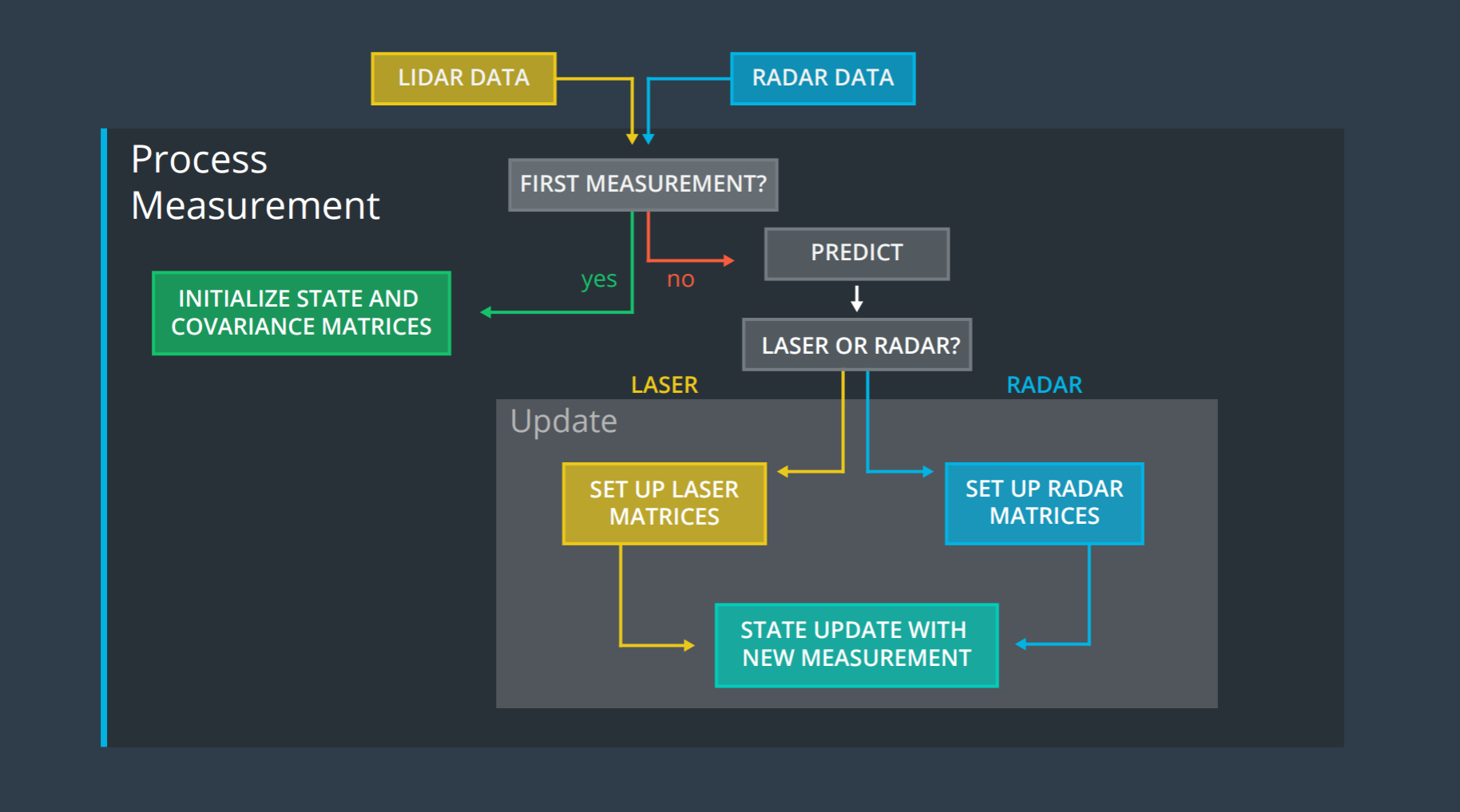
1. First measurement - receive initial measurements of the object's position, which usually comes from a ranger like a radar or lidar sensor
2. Initialize state and covariance matrices - the filter will initialize the object's position based on the first measurement
3. Predict - the algorithm will predict where the object will be after time Δt
4. Update - the filter compares the "predicted" location with what the sensor measurement says. The predicted location and the measured location are combined to give an updated location. The Kalman filter will put more weight on either the predicted location or the measured location depending on the uncertainty of each value.
5. receive another sensor measurement after a time period Δt. The algorithm then does another predict and update step.

 

Definition of Variables

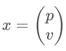
• x is the mean state vector. For an extended Kalman filter, the mean state vector contains information about the object's position and velocity that you are tracking. It is called the "mean" state vector because position and velocity are represented by a gaussian distribution with mean x.
• P is the state covariance matrix, which contains information about the uncertainty of the object's position and velocity. You can think of it as containing standard deviations.
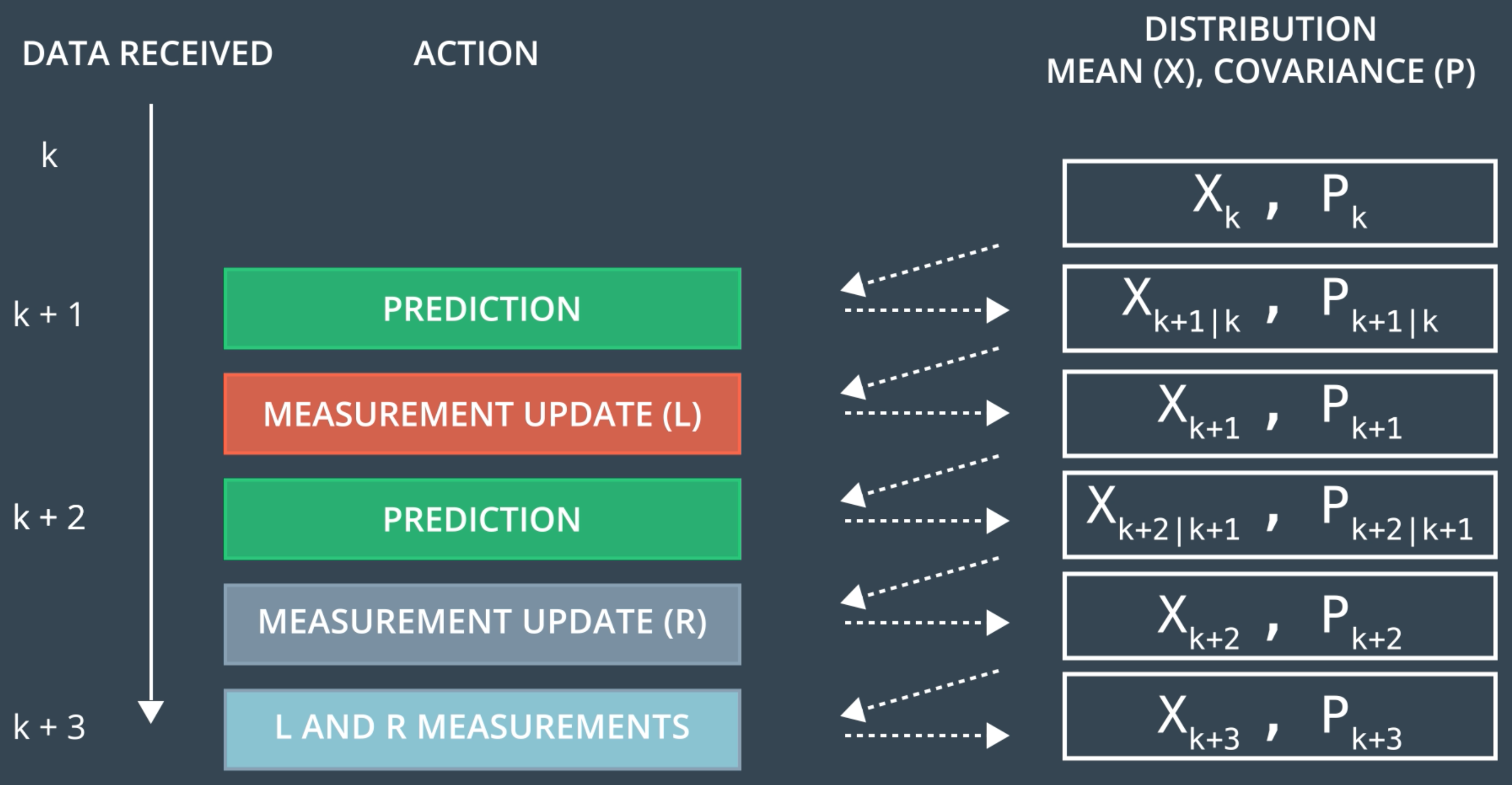
• k represents time steps. So x​k​​ refers to the object's position and velocity vector at time k.
• The notation ∣ refers to the prediction step. At time k+1, you receive a sensor measurement. Before taking into account the sensor measurement to update your belief about the object's position and velocity, you predict where you think the object will be at time k+1. You can predict the position of the object at k+1 based on its position and velocity at time k. Hence x​k+1∣k​​ means that you have predicted where the object will be at k+1 but have not yet taken the sensor measurement into account.
• x​k+1​​ means that you have now predicted where the object will be at time k+1 and then used the sensor measurement to update the object's position and velocity.

Prediction

Process noise refers to the uncertainty in the prediction step. We assume the object travels at a constant velocity, but in reality, the object might accelerate or decelerate. The notation ν∼N(0,Q) defines the process noise as a gaussian distribution with mean zero and covariance Q.

Update

Measurement noise refers to uncertainty in sensor measurements. The notation ω∼N(0,R) defines the measurement noise as a gaussian distribution with mean zero and covariance R. Measurement noise comes from uncertainty in sensor measurements.

Compare

Kalman Filter Gain

The K matrix, often called the Kalman filter gain, combines the uncertainty of where we think we are P​′​​ with the uncertainty of our sensor measurement R.

• If our sensor measurements are very uncertain (R is high relative to P'), then the Kalman filter will give more weight to where we think we are: x​′​​.
• If where we think we are is uncertain (P' is high relative to R), the Kalman filter will put more weight on the sensor measurement: z.

Why Bu is crossed out?

B is a matrix called the control input matrix and u is the control vector.

For the Kalman filter lessons, we will assume that there is no way to measure or know the exact acceleration of a tracked object. For example, if we were in an autonomous vehicle tracking a bicycle, pedestrian or another car, we would not be able to model the internal forces of the other object; hence, we do not know for certain what the other object's acceleration is. Instead, we will set Bu=0 and represent acceleration as a random noise with mean ν.

1) 1D Kalman Filter

Goal

To track an object, eg. a pedestrian with state x, which is described by a position and velocity.

Predict

The state transition function

By this function, we are representing the object location and velocity as gaussian distributions with mean x.

The noise is also represented by a gaussian distribution but with mean zero; hence, noise = 0 is saying that the mean noise is zero.

The noise does have uncertainty. The uncertainty shows up in the Q matrix as acceleration noise.

Update

The measurement function

General Algorithm

• a prediction step - predict the new state x and covariance P
• a measurement update (also called a correction step) - use the latest measurements to update the estimate and the uncertainty

2) 2D Kalman Filter

Laser mesurements

Variable Definitions

• z is the measurement vector.
  • For a lidar sensor, the z vector contains the position−x and position−y measurements.
• H is the matrix that projects your belief about the object's current state into the measurement space of the sensor.
  • For lidar, this is a fancy way of saying that we discard velocity information from the state variable since the lidar sensor only measures position: The state vector x contains information about [p​x​​,p​y​​,v​x​​,v​y​​] whereas the z vector will only contain [px,py]. Multiplying Hx allows us to compare x, our belief, with z, the sensor measurement.
• The prime notation in the x vector like p​x​′​​ means you have already done the prediction step but have not done the measurement step yet.
  • In other words, the object was at p​x​​. After time Δt, you calculate where you believe the object will be based on the motion model and get p​x​′​​.
• R - Measurement Noise Covariance Matrix
  • 
  • the matrix R represents the uncertainty in the position measurements we receive from the laser sensor
  • Generally, the parameters for the random noise measurement matrix will be provided by the sensor manufacturer.

Radar Measurement

• h(x) - Like the H matrix for the lidar, which is to solve y=z−Hx​′​​ in the update step, h(x) equations for the radar is actually accomplishing the same thing.

• For radar y=z−Hx​′​​ becomes y=z−h(x​′​​)
• For radar, there is no H matrix that will map the state vector x into polar coordinates. Instead, you need to calculate the mapping manually to convert from cartesian coordinates to polar coordinates.

Definition of Radar Variables

• The range, (ρ), is the distance to the pedestrian. The range is basically the magnitude of the position vector ρ which can be defined as ρ=sqrt(p​x​2​​+p​y​2​​).
• φ=atan(p​y​​/p​x​​). Note that φ is referenced counter-clockwise from the x-axis, so φ from the video clip above in that situation would actually be negative.
• The range rate, ​ρ​˙​​, is the projection of the velocity, v, onto the line, L.
• Since we have a nonlinear measurement function, h(x) , which cannot be applied with Gaussian Distribution, we cannot apply the Kalman Filter equations to update the predicted state, X, with new measurements, z.

3) Extended Kalman Filter

Taylor Expansion

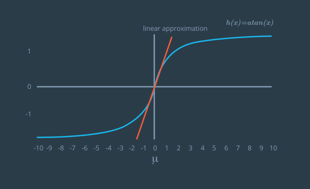
The general form of a Taylor series expansion of an equation, f(x), at point μ is as follows:

f(x)≈f(μ)+​∂x/​​∂f(μ)*​​(x−μ)

Use the first order Taylor expansion to construct a linear approximation of h(x) to find the equation of the line that linearizes the function h(x) at the mean location μ

Multivariate Taylor Series

Compared to Kalman Filters, the main differences of Extended Kalman Filter are:

• the F matrix will be replaced by F​j​​ when calculating P​′​​.
• the H matrix in the Kalman filter will be replaced by the Jacobian matrix H​j​​ when calculating S, K, and P.
• to calculate x​′​​, the prediction update function, f, is used instead of the F matrix.
• to calculate y, the h function is used instead of the H matrix.

To summarize:

• for measurement updates with lidar, we can use the H matrix for calculating y, S, K and P.
• for radar, H​j​​ is used to calculate S, K and P.