处理文本数据（下）：

4、停用词

删除没有信息量的单词还有另一种方法，就是舍弃那些出现次数太多以至于没有信息量的单词。有两种主要方法：使用特定语言的停用词（stopword）列表，或者舍弃那些出现过于频繁的单词。

• scikit-learn 的 feature_extraction.text 模块中提供了英语停用词的内置列表：

  from sklearn.feature_extraction.text import ENGLISH_STOP_WORDS

  print("Number of stop words: {}".format(len(ENGLISH_STOP_WORDS)))
  print("Every 10th stopword:\n{}".format(list(ENGLISH_STOP_WORDS)[::10]))


  # 指定 stop_words="english" 将使用内置列表
  # 我们也可以扩展这个列表并传入我们自己的列表
  vect = CountVectorizer(min_df=5, stop_words="english").fit(text_train)
  X_train = vect.transform(text_train)
  param_grid = {'C': [0.001, 0.01, 0.1, 1, 10]}

  print("X_train with stop words:\n{}".format(repr(X_train)))

  '''
  <25000x26966 sparse matrix of type '<class 'numpy.int64'>'
  	with 2149958 stored elements in Compressed Sparse Row format>
  '''


  #现在数据集中的特征数量减少了 305 个（27271-26966），说明大部分停用词（但不是所有）都出现了。我们再次运行网格搜索：

  grid = GridSearchCV(LogisticRegression(), param_grid, cv=5)
  grid.fit(X_train, y_train)
  print("Best cross-val上idation score: {:.2f}".format(grid.best_score_))
  # Best cross-validation score: 0.88

5、用 tf-idf 缩放数据

另一种方法是按照我们预计的特征信息量大小来缩放特征，而不是舍弃那些认为不重要的特征。
最常见的一种做法就是使用词频 - 逆向文档频率（term frequency–inverse document frequency，tf-idf）方法。

这一方法对在某个特定文档中经常出现的术语给予很高的权重，但对在语料库的许多文档中都经常出现的术语给予的权重却不高。
如果一个单词在某个特定文档中经常出现，但在许多文档中却不常出现，那么这个单词很可能是对文档内容的很好描述。

scikit-learn 在两个类中实现了 tf-idf 方法：TfidfTransformer 和 TfidfVectorizer，前者接受 CountVectorizer 生成的稀疏矩阵并将其变换，后者接受文本数据并完成词袋特征提取与 tf-idf 变换。

由于 tf-idf 实际上利用了训练数据的统计学属性，所以我们将使用管 道，以确保网格搜索的结果有效。这样会得到下列代码：

  from sklearn.feature_extraction.text import TfidfVectorizer
  from sklearn.pipeline import make_pipeline


  pipe = make_pipeline(TfidfVectorizer(min_df=5, norm=None),
                       LogisticRegression())
  param_grid = {'logisticregression__C': [0.001, 0.01, 0.1, 1, 10]}

  grid = GridSearchCV(pipe, param_grid, cv=5)
  grid.fit(text_train, y_train)
  print("Best cross-validation score: {:.2f}".format(grid.best_score_))
  # Best cross-validation score: 0.89

如你所见，使用 tf-idf 代替仅统计词数对性能有所提高。我们还可以查看 tf-idf 找到的最重要的单词。请记住，tf-idf 缩放的目的是找到能够区分文档的单词，但它完全是一种无监督技术。

因此，这里的 “重要” 不一定与我们感兴趣的 “正面评论” 和 “负面评论” 标签相关。

首先，我们从管道中提取 TfidfVectorizer：

  vectorizer = grid.best_estimator_.named_steps["tfidfvectorizer"]
  # 变换训练数据集
  X_train = vectorizer.transform(text_train)
  # 找到数据集中每个特征的最大值
  max_value = X_train.max(axis=0).toarray().ravel()
  sorted_by_tfidf = max_value.argsort()
  # 获取特征名称
  feature_names = np.array(vectorizer.get_feature_names())

  print("Features with lowest tfidf:\n{}".format(feature_names[sorted_by_tfidf[:20]]))
  '''
  Features with lowest tfidf:
  ['poignant' 'disagree' 'instantly' 'importantly' 'lacked' 'occurred'
   'currently' 'altogether' 'nearby' 'undoubtedly' 'directs' 'fond' 'stinker'
   'avoided' 'emphasis' 'commented' 'disappoint' 'realizing' 'downhill'
   'inane']
  '''
  print("Features with highest tfidf: \n{}".format(feature_names[sorted_by_tfidf[-20:]]))
  '''
  Features with highest tfidf: 
  ['coop' 'homer' 'dillinger' 'hackenstein' 'gadget' 'taker' 'macarthur'
   'vargas' 'jesse' 'basket' 'dominick' 'the' 'victor' 'bridget' 'victoria'
   'khouri' 'zizek' 'rob' 'timon' 'titanic']
  '''

tf-idf 较小的特征要么是在许多文档里都很常用，要么就是很少使用，且仅出现在非常长的文档中。

有趣的是，许多 tf-idf 较大的特征实际上对应的是特定的演出或电影。这些术语仅出现在这些特定演出或电影的评论中，但往往在这些评论中多次出现。例如，对于 “pokemon”、“smallville” 和 “doodlebops” 是显而易见的，但这里的 “scanners” 实际上指的也是电影标题。
这些单词不太可能有助于我们的情感分类任务（除非有些电影的评价可 能普遍偏正面或偏负面），但肯定包含了关于评论的大量具体信息。

6、研究模型系数

最后，我们详细看一下 Logistic 回归模型从数据中实际学到的内容。由于特征数量非常多 （删除出现次数不多的特征之后还有 27 271 个），所以显然我们不能同时查看所有系数。但 是，我们可以查看最大的系数，并查看这些系数对应的单词。我们将使用基于 tf-idf 特征训练的最后一个模型。

下面这张条形图给出了 Logistic 回归模型中最大的 25 个系数与最小的 25 个系数，其高度表示每个系数的大小：

  import mglearn

  mglearn.tools.visualize_coefficients(
      grid.best_estimator_.named_steps["logisticregression"].coef_,
      feature_names, n_top_features=40)

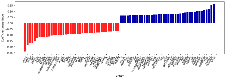
左侧的负系数属于模型找到的表示负面评论的单词，而右侧的正系数属于模型找到的表示正面评论的单词。

大多数单词都是非常直观的，比如 “worst”（最差）、“waste”（浪费）、“disappointment”（失望）和 “laughable”（可笑）都表示不好的电影评论，而 “excellent”（优秀）、“wonderful”（精彩）、“enjoyable”（令人愉悦）和 “refreshing” （耳目一新）则表示正面的电影评论。

有些词的含义不那么明确，比如 “bit”（一点）、 “job”（工作）和 “today”（今天），但它们可能是类似 “good job”（做得不错）和 “best today”（今日最佳）等短语的一部分。

7、多个单词的词袋（n 元分组）

使用词袋表示的主要缺点之一是完全舍弃了单词顺序。

因此，“it’s bad, not good at all”（电影很差，一点也不好）和 “it’s good, not bad at all”（电影很好，还不错）这两个字符串的词袋表示完全相同，尽管它们的含义相反。

将 “not”（不）放在单词前面，这只是上下文很重要的一个例子（可能是一个极端的例子）。

幸运的是，使用词袋表示时有一种获取上下文的方法，就是不仅考虑单一词例的计数，而且还考虑相邻的两个或三个词例的计数。

两个词例被称为二元分词（bigram），三个词例被称为三元分词（trigram），更一般的词例序列被称为 n 元分词（n-gram）。

我们可以通过改变 CountVectorizer 或 TfidfVectorizer 的 ngram_range 参数来改变作为特征的词例范围。

  #我们在 IMDb 电影评论数据上尝试使用 TfidfVectorizer，并利用网格搜索找出 n 元分词的最佳设置：

  pipe = make_pipeline(TfidfVectorizer(min_df=5), LogisticRegression())
  # 运行网格搜索需要很长的时间，因为网格相对较大，且包含三元分组
  param_grid = {'logisticregression__C': [0.001, 0.01, 0.1, 1, 10, 100],
                "tfidfvectorizer__ngram_range": [(1, 1), (1, 2), (1, 3)]}

  grid = GridSearchCV(pipe, param_grid, cv=5)
  grid.fit(text_train, y_train)
  print("Best cross-validation score: {:.2f}".format(grid.best_score_))
  # Best cross-validation score: 0.91
  print("Best parameters:\n{}".format(grid.best_params_))
  '''
  Best parameters:
  {'logisticregression__C': 100, 'tfidfvectorizer__ngram_range': (1, 3)}
  '''


  #将交叉验证精度作为 ngram_range 和 C 参数的函数并用热图可视化：

  # 从网格搜索中提取分数
  scores = grid.cv_results_['mean_test_score'].reshape(-1, 3).T
  # 热图可视化
  heatmap = mglearn.tools.heatmap(
      scores, xlabel="C", ylabel="ngram_range", cmap="viridis", fmt="%.3f",
      xticklabels=param_grid['logisticregression__C'],
      yticklabels=param_grid['tfidfvectorizer__ngram_range'])
  plt.colorbar(heatmap)

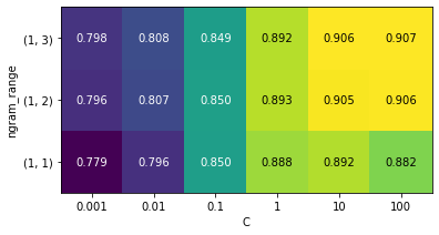
从热图中可以看出，使用二元分词对性能有很大提高，而添加三元分词对精度只有很小贡献。

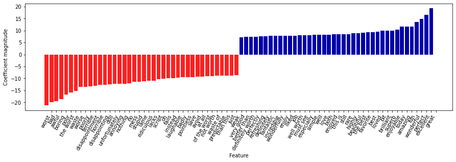
为了更好地理解模型是如何改进的，我们可以将最佳模型的重要系数可视化，其中包含一元分词、二元分词和三元分词：

8、主题建模与文档聚类

常用于文本数据的一种特殊技术是主题建模（topic modeling），这是描述将每个文档分配给一个或多个主题的任务（通常是无监督的）的概括性术语。这方面一个很好的例子是新闻数据，它们可以被分为 “政治” “体育” “金融” 等主题。

8.1、隐含狄利克雷分布

LDA 模型试图找出频繁共同出现的单词群组（即主题）。LDA 还要求，每个文档可以被理解为主题子集的 “混合”。重要的是要理解，机器学习模型所谓的 “主题” 可能不是我们通常在日常对话中所说的主题，而是更类似于 PCA 或 NMF所提取的成分，它可能具有语义，也可能没有。

我们将 LDA 应用于电影评论数据集，来看一下它在实践中的效果。对于无监督的文本文档模型，通常最好删除非常常见的单词，否则它们可能会支配分析过程。我们将删除至少在 15% 的文档中出现过的单词，并在删除前 15% 之后，将词袋模型限定为最常见的 10 000 个单词：

  vect = CountVectorizer(max_features=10000, max_df=.15)
  X = vect.fit_transform(text_train)

  from sklearn.decomposition import LatentDirichletAllocation
  lda = LatentDirichletAllocation(n_topics=10, learning_method="batch",
                                  max_iter=25, random_state=0)
  #我们在一个步骤中构建模型并变换数据
  #计算变换需要花点时间，二者同时进行可以节省时间
  document_topics = lda.fit_transform(X)


  print("lda.components_.shape: {}".format(lda.components_.shape))
  
  '''
  lda.components_.shape: (10, 10000)
  '''
  #对于每个主题（components_的一行），将特征排序（升序）
  #用[:, ::-1]将行反转，使排序变为降序
  sorting = np.argsort(lda.components_, axis=1)[:, ::-1]
  #从向量器中获取特征名称
  feature_names = np.array(vect.get_feature_names())

  #打印出前10个主题：
  mglearn.tools.print_topics(topics=range(10), feature_names=feature_names,
                             sorting=sorting, topics_per_chunk=5, n_words=10)
  
  '''
  '''
  topic 0       topic 1       topic 2       topic 3       topic 4       
  --------      --------      --------      --------      --------      
  between       war           funny         show          didn          
  family        world         comedy        series        saw           
  young         us            guy           episode       thought       
  real          american      laugh         tv            am            
  us            our           jokes         episodes      thing         
  director      documentary   fun           shows         got           
  work          history       humor         season        10            
  both          years         re            new           want          
  beautiful     new           hilarious     years         going         
  each          human         doesn         television    watched       


  topic 5       topic 6       topic 7       topic 8       topic 9       
  --------      --------      --------      --------      --------      
  action        kids          role          performance   horror        
  effects       action        cast          role          house         
  nothing       animation     john          john          killer        
  budget        children      version       actor         gets          
  script        game          novel         cast          woman         
  minutes       disney        director      plays         dead          
  original      fun           both          jack          girl          
  director      old           played        michael       around        
  least         10            mr            oscar         goes          
  doesn         kid           young         father        wife
  '''
  '''

  lda100 = LatentDirichletAllocation(n_topics=100, learning_method="batch",
                                     max_iter=25, random_state=0)
  document_topics100 = lda100.fit_transform(X)

  #查看所有 100 个主题可能有点困难，所以我们选取了一些有趣的而且有代表性的主题：

  topics = np.array([7, 16, 24, 25, 28, 36, 37, 41, 45, 51, 53, 54, 63, 89, 97])
  sorting = np.argsort(lda100.components_, axis=1)[:, ::-1]
  feature_names = np.array(vect.get_feature_names())
  mglearn.tools.print_topics(topics=topics, feature_names=feature_names,
                             sorting=sorting, topics_per_chunk=5, n_words=20)

  '''
  '''
  topic 7       topic 16      topic 24      topic 25      topic 28      
  --------      --------      --------      --------      --------      
  thriller      worst         german        car           beautiful     
  suspense      awful         hitler        gets          young         
  horror        boring        nazi          guy           old           
  atmosphere    horrible      midnight      around        romantic      
  mystery       stupid        joe           down          between       
  house         thing         germany       kill          romance       
  director      terrible      years         goes          wonderful     
  quite         script        history       killed        heart         
  bit           nothing       new           going         feel          
  de            worse         modesty       house         year          
  performances  waste         cowboy        away          each          
  dark          pretty        jewish        head          french        
  twist         minutes       past          take          sweet         
  hitchcock     didn          kirk          another       boy           
  tension       actors        young         getting       loved         
  interesting   actually      spanish       doesn         girl          
  mysterious    re            enterprise    now           relationship  
  murder        supposed      von           night         saw           
  ending        mean          nazis         right         both          
  creepy        want          spock         woman         simple        


  topic 36      topic 37      topic 41      topic 45      topic 51      
  --------      --------      --------      --------      --------      
  performance   excellent     war           music         earth         
  role          highly        american      song          space         
  actor         amazing       world         songs         planet        
  cast          wonderful     soldiers      rock          superman      
  play          truly         military      band          alien         
  actors        superb        army          soundtrack    world         
  performances  actors        tarzan        singing       evil          
  played        brilliant     soldier       voice         humans        
  supporting    recommend     america       singer        aliens        
  director      quite         country       sing          human         
  oscar         performance   americans     musical       creatures     
  roles         performances  during        roll          miike         
  actress       perfect       men           fan           monsters      
  excellent     drama         us            metal         apes          
  screen        without       government    concert       clark         
  plays         beautiful     jungle        playing       burton        
  award         human         vietnam       hear          tim           
  work          moving        ii            fans          outer         
  playing       world         political     prince        men           
  gives         recommended   against       especially    moon          


  topic 53      topic 54      topic 63      topic 89      topic 97      
  --------      --------      --------      --------      --------      
  scott         money         funny         dead          didn          
  gary          budget        comedy        zombie        thought       
  streisand     actors        laugh         gore          wasn          
  star          low           jokes         zombies       ending        
  hart          worst         humor         blood         minutes       
  lundgren      waste         hilarious     horror        got           
  dolph         10            laughs        flesh         felt          
  career        give          fun           minutes       part          
  sabrina       want          re            body          going         
  role          nothing       funniest      living        seemed        
  temple        terrible      laughing      eating        bit           
  phantom       crap          joke          flick         found         
  judy          must          few           budget        though        
  melissa       reviews       moments       head          nothing       
  zorro         imdb          guy           gory          lot           
  gets          director      unfunny       evil          saw           
  barbra        thing         times         shot          long          
  cast          believe       laughed       low           interesting   
  short         am            comedies      fulci         few           
  serial        actually      isn           re            half
  '''
  '''

在没有标签的情况下（或者像本章的例子这样，即使有标签的情况下），像 LDA 这样的主 题模型是理解大型文本语料库的有趣方法。不过 LDA 算法是随机的，改变 random_state 参数可能会得到完全不同的结果。虽然找到主题可能很有用，但对于从无监督模型中得出的任何结论都应该持保留态度，我们建议通过查看特定主题中的文档来验证你的直觉。 LDA.transform 方法生成的主题有时也可以用于监督学习的紧凑表示。当训练样例很少时， 这一方法特别有用。

参考文献

《机器学习基础教程》