
深度学习入门书籍笔记
第3章 神经网络
3.2 激活函数
将输入信号的总和转换为输出信号,一般称为激活函数
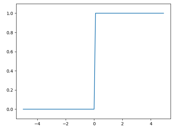
3.2.3 阶跃函数的图形
p44
import numpy as np
import matplotlib.pyplot as plt

def step_function(x):
    return np.array(x > 0,dtype=np.int)

x = np.arange(-5.0,5.0,0.1)
y = step_function(x)
plt.plot(x,y)
plt.ylim(-0.1,1.1)
plt.show()
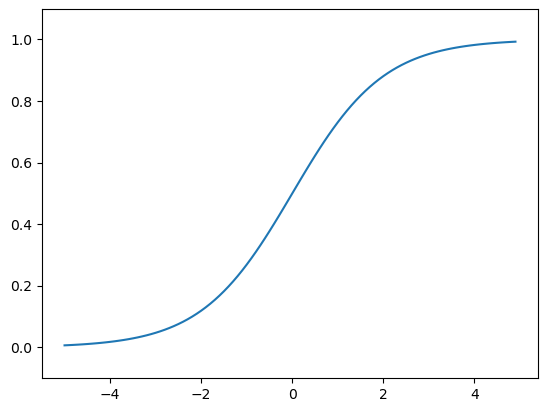
3.2.4 sigmoid函数实现
p45
sigmoid函数也叫Logistic函数,用于隐层神经元输出,取值范围为(0,1),它可以将一个实数映射到(0,1)的区间
import numpy as np
from matplotlib import pyplot as plt


def sigmoid(x):
    return 1 / (1 + np.exp(-x))

x = np.array([-1.0,1.0,2.0])
print(sigmoid(x)) # [0.26894142 0.73105858 0.88079708]

x = np.arange(-5.0,5.0,0.1)
y = sigmoid(x)
plt.plot(x,y)
plt.ylim(-0.1,1.1)
plt.show()
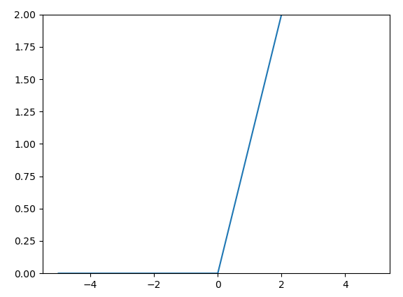
3.2.7 ReLu函数
p49
import numpy as np
from matplotlib import pyplot as plt


def relu(x):
    return np.maximum(0,x)

x = np.arange(-5.0,5.0,0.1)
y = relu(x)
plt.plot(x,y)
plt.ylim(0,2)
plt.show()
3.3 多维数组的运算
3.3.1 多维数组
p50
import numpy as np
A = np.array([1,2,3,4])
print(np.ndim(A)) # 1

print(A.shape) # (4,)

print(A.shape[0]) # 4

B = np.array([[1,2],[3,4],[5,6]])
print(B)
# [[1 2]
#  [3 4]
#  [5 6]]

print(np.ndim(B)) # 2

print(B.shape) # (3, 2)
3.3.2 矩阵乘法
p52
import numpy as np

A = np.array([[1,2],[3,4]])
print(A.shape) # (2, 2)

B = np.array([[5,6],[7,8]])
print(B.shape) # (2, 2)

print(np.dot(A,B))
# [[19 22]
#  [43 50]]
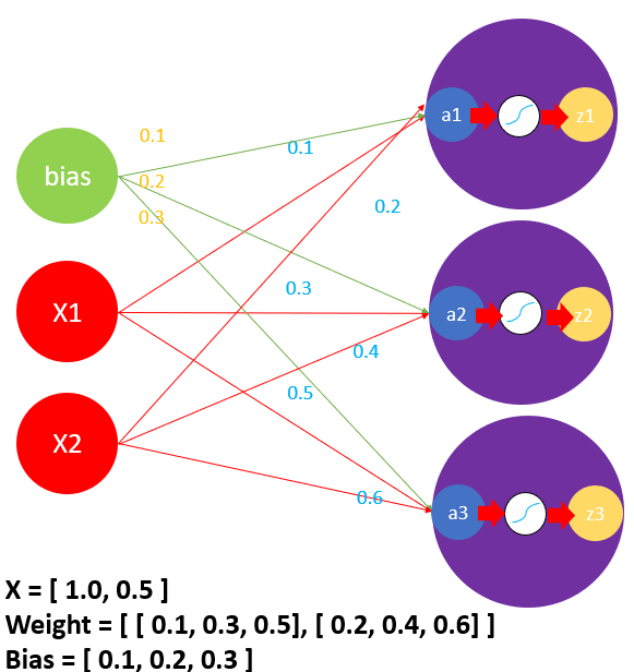
3.4 3层神经网络实现
p62
一层神经网络
代码实现
import numpy as np

def sigmoid(x):
    return 1 / (1 + np.exp(-x))

X = np.array([1.0,0.5])
W1 = np.array([[0.1,0.3,0.5],[0.2,0.4,0.6]])
B1 = np.array([0.1,0.2,0.3])

print(W1.shape) # (2, 3)
print(B1.shape) # (3,)
print(X.shape) # (2,)

A1 = np.dot(X,W1) + B1
print(A1) #[0.3 0.7 1.1]

Z1 = sigmoid(A1)
print(Z1) # [0.57444252 0.66818777 0.75026011]
3层代码实现
import numpy as np

def sigmoid(x):
    return 1 / (1 + np.exp(-x))

# identity_function也称恒等函数,没有特定意义,只是为了之前的流程保持一致
def identity_function(x):
    return x

def init_network():
    network = {}
    network['W1'] = np.array([[0.1,0.3,0.5],[0.2,0.4,0.6]])
    network['B1'] = np.array([0.1,0.2,0.3])
    network['W2'] = np.array([[0.1,0.4],[0.2,0.5],[0.3,0.6]])
    network['B2'] = np.array([0.1,0.2])
    network['W3'] = np.array([[0.1,0.3],[0.2,0.4]])
    network['B3'] = np.array([0.1,0.2])

    return network

def forward(network,X):
    W1,W2,W3 = network['W1'],network['W2'],network['W3']
    B1,B2,B3 = network['B1'],network['B2'],network['B3']

    # 第一层
    a1 = np.dot(X,W1) + B1
    z1 = sigmoid(a1)
    # 第二层
    a2 = np.dot(z1,W2) + B2
    z2 = sigmoid(a2)
    # 第三层
    a3 = np.dot(z2,W3) + B3
    y = identity_function(a3)

    return y

network = init_network()
x = np.array([1.0,0.5])
y = forward(network,x)

print(y)  # [0.31682708 0.69627909]
init_work()函数会进行权重和偏置值的初始化,并保存到字典变量network中
forward()函数封装输入信号到输出信号的处理过程,forward一词表示从输入到输出方向的传递过程,和backward相反
3.5 输出层的设计
3.5.1 softmax函数实现
p64
# 普通版本
def softmax(a):
    x = np.exp(a)
    sum = np.sum(x)
    return x / sum

# 防溢出版本 p67
def softmax(a):
    c = np.max(a)
    exp_a = np.exp(a - c) # 溢出对策
    sum_exp_a = np.sum(exp_a)
    y = exp_a / sum_exp_a

    return y

print(softmax(np.array([0.3,2.9,4.0]))) # [0.01821127 0.24519181 0.73659691]
softmax()函数的输出是0.0到1.0之间的实数,并且softmax()函数的输出值的总和是1,所以才可以把softmax()函数的输出解释为”概率“,输出结果的第一个可以理解为概率为1.8%,第二个为25%,第三个为74%
3.6 手写数字识别
3.6.1 mnist数据集
p70
import sys,os
sys.path.append(os.pardir)
from dataset.mnist import load_mnist

(x_train,t_train),(x_test,t_test) = load_mnist(flatten=True,normalize=False)

print(x_train.shape) # (60000, 784)
print(t_train.shape) # (60000,)
print(x_test.shape) # (10000, 784)
print(t_test.shape) # (10000,)
print(np.ndim(x_train)) # 2
load_mnis()函数以(训练图像,训练标签),(测试图像,测试标签)为返回值
normalize设置是否将输入图像正规化为0.01.0的值,如果为False,则输入图像会保持原来的0255
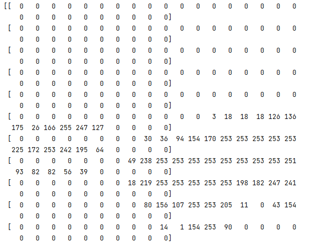
flatten设置是否展开图像(变为一维数组),如果设为False,输出1×28×28的三维数组,设为True,输出784个元素构成的一维数组
x_train的输出
显示图片
import sys,os
sys.path.append(os.pardir)
import numpy as np
from dataset.mnist import load_mnist
from PIL import Image

def img_show(img):
    pil_img = Image.fromarray(np.uint8(img))
    pil_img.show()

(x_train,t_train),(x_test,t_test) = load_mnist(flatten=True,normalize=False)
img = x_train[0]
label = t_train[0]
print(label) #5

print(img.shape) # (784,)
img = img.reshape(28,28)
print(img.shape) # (28, 28)

img_show(img)
img矩阵(部分)shape为(784,)
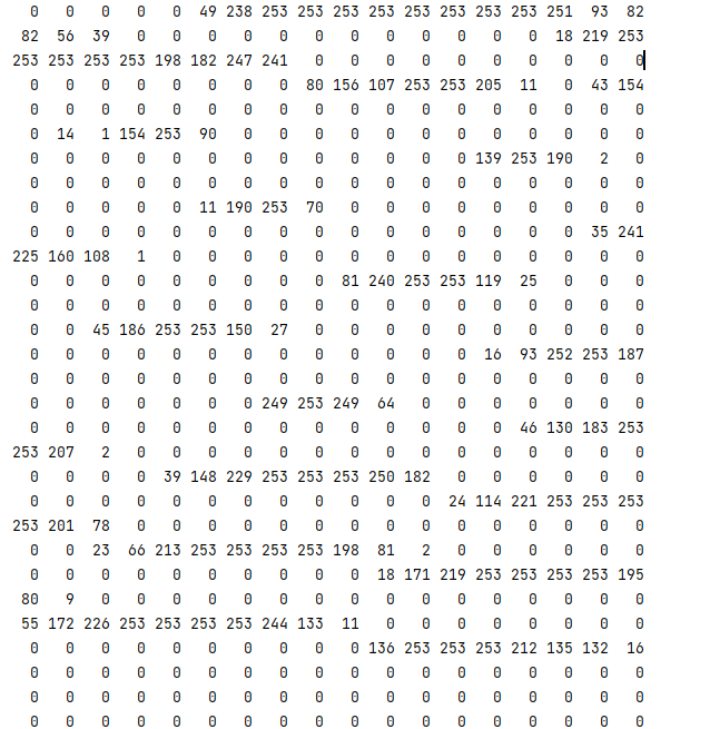
img矩阵(部分)shape为(28, 28)
3.6.3 批处理
p77
# coding: utf-8
import sys, os
sys.path.append(os.pardir)  # 为了导入父目录的文件而进行的设定
import numpy as np
import pickle
from dataset.mnist import load_mnist
from common.functions import sigmoid, softmax


def get_data():
    (x_train, t_train), (x_test, t_test) = load_mnist(normalize=True, flatten=True, one_hot_label=False)
    return x_test, t_test


def init_network():
    with open("sample_weight.pkl", 'rb') as f:
        network = pickle.load(f)
    return network


def predict(network, x):
    w1, w2, w3 = network['W1'], network['W2'], network['W3']
    b1, b2, b3 = network['b1'], network['b2'], network['b3']

    a1 = np.dot(x, w1) + b1
    z1 = sigmoid(a1)
    a2 = np.dot(z1, w2) + b2
    z2 = sigmoid(a2)
    a3 = np.dot(z2, w3) + b3
    y = softmax(a3)

    return y


x, t = get_data()
print(x.shape) # (10000, 784)
network = init_network()
print(network)

batch_size = 100 # 批数量
accuracy_cnt = 0

for i in range(0, len(x), batch_size):
    x_batch = x[i:i+batch_size]
    print(x_batch.shape) # (100, 784) # 100个矩阵,每个矩阵里面784个元素
    y_batch = predict(network, x_batch)
    p = np.argmax(y_batch, axis=1)
    accuracy_cnt += np.sum(p == t[i:i+batch_size])

print("Accuracy:" + str(float(accuracy_cnt) / len(x)))
第4章 神经网络的学习
4.2 损失函数
4.2.1 均方误差
p86
import numpy as np

def mean_squared_error(y,t):
    return 0.5 * np.sum((y-t)**2)
y = [0.1,0.05,0.6,0.0,0.05,0.1,0.0,0.1,0.0,0.0,0.0]
t = [0,0,0,1,0,0,0,0,0,0,0]

print(mean_squared_error(np.array(y),np.array(t))) # 0.6974999999999999
4.2.2 交叉熵误差
p87
import numpy as np

def cross_entroy_error(y,t):
    delta = 1e-7 # 防止除数为0,防止分母为0
    return -np.sum(t * np.log(y + delta))
4.2.3 mini-batch学习
这里损失函数以交叉熵为例,可以写成下面的式子
假设batch大小为N,算出误差后,最后还要除以N,进行正则化。通过除以N,可以求得单个数据的“平均损失函数”。通过这样的平均化,可以获得和训练数据的数量无关的统一指标。
p89
如果数据很大,我们从全部数据中选出一部分,作为全部数据的”近似“,神经网络学习也是从训练数据中选出一批数据(称为mini-batch批量),然后对这个批量进行学习。比如,从60000个训练数据中,随机选择100笔,再用这个100笔进行学习,这种学习方式就是mini-batch学习
import sys,os
sys.path.append(os.pardir)
import numpy as np
from dataset.mnist import load_mnist

(x_train,t_train),(x_test,t_test) = load_mnist(normalize=True,one_hot_label=True)

print(x_train.shape) # (60000, 784)
print(t_train.shape) # (60000, 10)

###### 随机挑选10个 #######
train_size = x_train.shape[0] # 60000
batch_size = 10
batch_mask = np.random.choice(train_size,batch_size)
x_batch = x_train[batch_mask]
t_batch = t_train[batch_mask]
np.random.choice(a,b) :从a中挑选b个数据
4.2.4 mini-batch版交叉熵实现
p91
当y的纬度是1时,即求单个数据的交叉熵误差时,需要改变数据的形状。并且当输入是mini-batch时,要用batch的个数进行正规化,计算单个数据的平均交叉熵误差
监督数据是one-hot形式
import numpy as np

def cross_entroy_error_mini_batch(y,t):
    if y.ndim == 1:
        t = t.reshape(1,t.shape)
        y = y.reshape(1,y.shape)

    batch_size = y.shape(1,t.size)
    return -np.sum(t * np.log(y + 1e-7)) / batch_size


t = np.array([1,2,3])

print(np.ndim(t))  # 1
print(t) # [1 2 3]
print(t.shape) # (3,)

t = t.reshape(1,t.size)
print(t) # [[1 2 3]]
print(t.shape) # (1, 3)
监督数据是标签形式(非one-hot形式,而是像”2“,”7“,”8“)
def cross_entropy_error_mini_batch_label(y,t):
    if y.ndim == 1:
        t = t.reshape(1,t.size)
        y = y.reshape(1,y.size)

    batch_size = y.shape[0]
    return -np.sum(np.log(y[np.arange(batch_size),t]+1e-7)) / batch_size
np.arange(batch_size):会返回0到batch_size-1的数组
t中的标签是以[2,7,0,9,4]的形式存储的,所以y[np.arange(batch_size),t]能抽出各个数据的正确解标签对应的神经网络的输出,这里生成numpy数组[y[0,2],y[1,7],y[2,0],y[3,9],y[4,4]]
4.3 数值微分
4.3.1 导数
p95
import numpy as np
from matplotlib import pyplot as plt


def numerical_diff(f,x):
    h = 1e-4 # 0.0001
    return (f(x+h) - f(x-h)) / (2*h)

def function_1(x):
    return x**2

x = np.arange(0.0,20.0,0.1) # 以0.1为刻度单位,从0到20的数组
y = function_1(x)
plt.xlabel("x")
plt.ylabel("y")
plt.plot(x,y)
plt.show()

# 计算y=x^2在x=2处的导数

print(numerical_diff(function_1,2)) # 4.000000000004
4.4 梯度
p101
import numpy as np

# y = x1^2+x2^2
def function_2(x):
    return x[0]**2+x[1]**2

def numerical_gradient(f,x):
    h = 1e-4 # 0.0001
    grad = np.zeros_like(x) # 生成和x形状相同的数组

    for idx in range(x.size):
        tmp_val = x[idx]
        # f(x+h)的计算
        x[idx] = tmp_val + h
        fxh1 = f(x)

        # f(x-h)的计算
        x[idx] = tmp_val - h
        fxh2 = f(x)

        grad[idx] = (fxh1 -fxh2) / (2*h)
        x[idx] = tmp_val # 还原值

    return grad

x = np.array([3.0,4.0])
# 计算 y = x1^2+x2^2 在(3,4)位置的导数
print(numerical_gradient(function_2,x)) # [6. 8.]
4.4.1 梯度下降法
p105
import numpy as np
from matplotlib import pyplot as plt


def function_2(x):
    return x[0]**2 + x[1]**2

def numerical_gradient(f,x):
    h = 1e-4
    grad = np.zeros_like(x)

    for idx in range(x.size):
        tmp_val = x[idx]
        x[idx] = tmp_val + h
        fxh1 = f(x)

        x[idx] = tmp_val - h
        fxh2 = f(x)

        grad[idx] = (fxh1 - fxh2) / (2*h)

    return grad


def gradient_descent(f,init_x,lr=0.01,step_num=100):
    x = init_x
    x_history = []
    for i in range(step_num):
        x_history.append(x.copy())
        grad = numerical_gradient(f,x)
        x -= lr*grad

    return x,np.array(x_history)

x, x_history = gradient_descent(function_2, np.array([-3.0, 4.0]))

plt.plot( [-5, 5], [0,0], '--b')
plt.plot( [0,0], [-5, 5], '--b')
plt.plot(x_history[:,0], x_history[:,1], 'o')

plt.xlim(-3.5, 3.5)
plt.ylim(-4.5, 4.5)
plt.xlabel("X0")
plt.ylabel("X1")
plt.show()
X[:,0]是numpy中数组的一种写法,表示对一个二维数组,取该二维数组第一维中的所有数据,第二维中取第0个数据,直观来说,X[:,0]就是取所有行的第0个数据, X[:,1] 就是取所有行的第1个数据。
如果要找最低点,用梯度下降,找最高点,用梯度上升法
4.4.2 神经网络的梯度
p107
import sys,os
import time

sys.path.append(os.pardir)
import numpy as np

def cross_entropy_error(y, t):
    if y.ndim == 1:  # 如果不进行转换,后面很多操作无法进行下去
        t = t.reshape(1, t.size)
        y = y.reshape(1, y.size)

    # 监督数据是one-hot-vector的情况下,转换为正确解标签的索引
    if t.size == y.size:
        t = t.argmax(axis=1)

    batch_size = y.shape[0]
    return -np.sum(np.log(y[np.arange(batch_size), t] + 1e-7)) / batch_size

def softmax(x):
    if x.ndim == 2:
        x = x.T
        x = x - np.max(x, axis=0)
        y = np.exp(x) / np.sum(np.exp(x), axis=0)
        return y.T

    x = x - np.max(x) # 溢出对策
    return np.exp(x) / np.sum(np.exp(x))

def numerical_gradient(f, x):
    h = 1e-4  # 0.0001
    grad = np.zeros_like(x)

    it = np.nditer(x, flags=['multi_index'], op_flags=['readwrite'])
    while not it.finished:
        idx = it.multi_index
        tmp_val = x[idx]
        x[idx] = float(tmp_val) + h
        fxh1 = f(x)  # f(x+h)

        x[idx] = tmp_val - h
        fxh2 = f(x)  # f(x-h)
        grad[idx] = (fxh1 - fxh2) / (2 * h)

        x[idx] = tmp_val  # 还原值
        it.iternext()

    return grad

class SimpleNet:
    def __init__(self):
        self.W = np.random.randn(2,3) # 用高斯分布进行初始化

    def predict(self,x):
        return np.dot(x,self.W)

    def loss(self,x,t):
        z = self.predict(x)
        y = softmax(z)
        loss = cross_entropy_error(y,t)

        return loss

# 参数测试用
t = np.array([1,2,3])
# print(t.argmax(axis=1)) numpy.AxisError: axis 1 is out of bounds for array of dimension 1  报错不能,执行,需要进行reshape后才能运行
print(np.ndim(t))  # 1
print(t) # [1 2 3]
print(t.shape) # (3,)

# 参数测试用
t = t.reshape(1,t.size)
print(t) # [[1 2 3]]
print(t.shape) # (1, 3)
print(t.argmax(axis=1)) # 2

net = SimpleNet()
print(net.W) # 权重参数
x = np.array([0.6,0.9])
p = net.predict(x)
print(p)
print(np.argmax(p))  # 2
print(np.ndim(p))    # 1

t = np.array([0,0,1])
net.loss(x,t)
4.5 学习算法的实现
p109
神经网络学习分为4个步骤
步骤1(mini-batch)
从训练数据中随机挑选一部分数据
步骤2(计算梯度)
为了减少mini-batch的损失函数的值,需要求出各个权重参数的梯度。梯度表示损失函数的值减少最多的方向
步骤3(更新参数)
将权重参数沿梯度方向进行微小更新
步骤4(重复)
重复上述步骤
4.5.1 2层神经网络的分类
p111
import sys,os

import numpy as np

sys.path.append(os.pardir)
from common.functions import *
from common.gradient import numerical_gradient

class TwoLayerNet:

    def __init__(self,input_size,hidden_size,output_size,weight_init_std=0.01):
        # 初始化权重
        self.params = {}
        self.params['W1'] = weight_init_std * np.random.randn(input_size,hidden_size)
        self.params['b1'] = np.zeros(hidden_size)

        self.params['W2'] = weight_init_std * np.random.randn(hidden_size,output_size)
        self.params['b2'] = np.zeros(output_size)

    def predict(self,x):
        W1,W2 = self.params['W1'],self.params['W2']
        b1,b2 = self.params['b1'],self.params['b2']

        a1 = np.dot(x,W1) + b1
        z1 = sigmoid(a1)
        a2 = np.dot(z1,W2) + b2
        y = softmax(a2)

        return y

    # x:输入数据。t:监督数据
    def loss(self,x,t):
        y = self.predict(x)
        return cross_entropy_error(y,t)

    def accuracy(self,x,t):
        y = self.predict(x)
        y = np.argmax(y,axis=1)
        t = np.argmax(t,axis=1)

        accuracy = np.sum(y == t) / float(x.shape[0])
        return accuracy

    # x:输入数据,t:监督数据
    def numerical_gradient(self,x,t):
        loss_W = lambda W:self.loss(x,t)

        grads = {}
        grads['W1'] = numerical_gradient(loss_W,self.params['W1'])
        grads['b1'] = numerical_gradient(loss_W,self.params['b1'])
        grads['W2'] = numerical_gradient(loss_W,self.params['W2'])
        grads['b2'] = numerical_gradient(loss_W,self.params['b2'])

        return grads

net = TwoLayerNet(input_size=784,hidden_size=100,output_size=10)
print(net.params['W1'].shape) #(784, 100)
print(net.params['b1'].shape) #(100,)
print(net.params['W2'].shape) #(100, 10)
print(net.params['b2'].shape) #(10,)


x = np.random.randn(100,784) # 伪输入数据(100笔)
t = np.random.randn(100,10)  # 伪正确数(100笔)

grads = net.numerical_gradient(x,t)
print(grads['W1'].shape) #(784, 100)
print(grads['b1'].shape)#(100,)
print(grads['W2'].shape) #(100, 10)
print(grads['b2'].shape)#(10,)
input_size:输入层的神经元数,输入图像大小是784(28×28)
hidden_size:隐藏层的神经元数,将隐藏层的个数设置一个合适的值就可以了
output_size:输出层的神经元数,输出为10个类别
np.random.randn(m,n):生成m×n的矩阵
4.5.2 mini-batch实现
p115
mini-batch设为100,每次从60000个数据选100个出来,执行10000次。每更新一次,都对训练数据计算损失函数的值,并添加到数组中。
import sys,os

import numpy as np
from torch import nn

sys.path.append(os.pardir)
from common.functions import *
from common.gradient import numerical_gradient
from dataset.mnist import load_mnist

import torch

class TwoLayerNet:

    def __init__(self,input_size,hidden_size,output_size,weight_init_std=0.01):

        # 初始化权重
        self.params = {}
        self.params['W1'] = weight_init_std * np.random.randn(input_size,hidden_size)
        self.params['b1'] = np.zeros(hidden_size)

        self.params['W2'] = weight_init_std * np.random.randn(hidden_size,output_size)
        self.params['b2'] = np.zeros(output_size)

    def predict(self,x):
        W1,W2 = self.params['W1'],self.params['W2']
        b1,b2 = self.params['b1'],self.params['b2']
        a1 = np.dot(x,W1) + b1
        z1 = sigmoid(a1)
        a2 = np.dot(z1,W2) + b2
        y = softmax(a2)

        return y

    # x:输入数据。t:监督数据
    def loss(self,x,t):
        y = self.predict(x)
        return cross_entropy_error(y,t)

    def accuracy(self,x,t):
        y = self.predict(x)
        y = np.argmax(y,axis=1)
        t = np.argmax(t,axis=1)

        accuracy = np.sum(y == t) / float(x.shape[0])
        return accuracy

    # x:输入数据,t:监督数据
    def numerical_gradient(self,x,t):
        loss_W = lambda W:self.loss(x,t)

        grads = {}
        grads['W1'] = numerical_gradient(loss_W,self.params['W1'])
        grads['b1'] = numerical_gradient(loss_W,self.params['b1'])
        grads['W2'] = numerical_gradient(loss_W,self.params['W2'])
        grads['b2'] = numerical_gradient(loss_W,self.params['b2'])

        return grads

(x_train,t_train),(x_test,t_test) = load_mnist(normalize=True,one_hot_label=True)

train_loss_list = []

# 超参数
iters_num = 10000
train_size = x_train.shape[0]
batch_size = 100
learning_rate = 0.1
network = TwoLayerNet(input_size=784,hidden_size=50,output_size=10)

for i in range(iters_num):
    # 获取mini-batch
    batch_mask = np.random.choice(train_size,batch_size)
    x_batch = x_train[batch_mask]
    t_batch = t_train[batch_mask]

    # 计算梯度
    grad = network.numerical_gradient(x_batch,t_batch)

    # 更新参数
    for key in ('W1','b1','W2','b2'):
        network.params[key] -= learning_rate * grad[key]

    # 记录学习过程
    loss = network.loss(x_batch,t_batch).cuda()
    train_loss_list.append(loss)
4.5.3 基于测试数据的评价
p117
import sys,os

import numpy as np
from torch import nn

sys.path.append(os.pardir)
from common.functions import *
from common.gradient import numerical_gradient
from dataset.mnist import load_mnist

import torch

class TwoLayerNet:

    def __init__(self,input_size,hidden_size,output_size,weight_init_std=0.01):

        # 初始化权重
        self.params = {}
        self.params['W1'] = weight_init_std * np.random.randn(input_size,hidden_size)
        self.params['b1'] = np.zeros(hidden_size)

        self.params['W2'] = weight_init_std * np.random.randn(hidden_size,output_size)
        self.params['b2'] = np.zeros(output_size)

    def predict(self,x):
        W1,W2 = self.params['W1'],self.params['W2']
        b1,b2 = self.params['b1'],self.params['b2']
        a1 = np.dot(x,W1) + b1
        z1 = sigmoid(a1)
        a2 = np.dot(z1,W2) + b2
        y = softmax(a2)

        return y

    # x:输入数据。t:监督数据
    def loss(self,x,t):
        y = self.predict(x)
        return cross_entropy_error(y,t)

    def accuracy(self,x,t):
        y = self.predict(x)
        y = np.argmax(y,axis=1)
        t = np.argmax(t,axis=1)

        accuracy = np.sum(y == t) / float(x.shape[0])
        return accuracy

    # x:输入数据,t:监督数据
    def numerical_gradient(self,x,t):
        loss_W = lambda W:self.loss(x,t)

        grads = {}
        grads['W1'] = numerical_gradient(loss_W,self.params['W1'])
        grads['b1'] = numerical_gradient(loss_W,self.params['b1'])
        grads['W2'] = numerical_gradient(loss_W,self.params['W2'])
        grads['b2'] = numerical_gradient(loss_W,self.params['b2'])

        return grads

(x_train,t_train),(x_test,t_test) = load_mnist(normalize=True,one_hot_label=True)

train_loss_list = []
train_acc_list = []
test_acc_list = []


# 超参数
iters_num = 10000
train_size = x_train.shape[0]
batch_size = 100
learning_rate = 0.1

# 平均每个epoch的重复次数
iter_per_epoch = max(train_size / batch_size,1)

network = TwoLayerNet(input_size=784,hidden_size=50,output_size=10)

for i in range(iters_num):
    print("第{}次".format(i))
    # 获取mini-batch
    batch_mask = np.random.choice(train_size,batch_size)
    x_batch = x_train[batch_mask]
    t_batch = t_train[batch_mask]

    # 计算梯度
    grad = network.numerical_gradient(x_batch,t_batch)
    print(grad)
    # 更新参数
    for key in ('W1','b1','W2','b2'):
        network.params[key] -= learning_rate * grad[key]

    # 记录学习过程
    loss = network.loss(x_batch,t_batch)
    train_loss_list.append(loss)

    # 计算每个epoch的识别精度
    if i % iter_per_epoch == 0:
        train_acc = network.accuracy(x_train,t_train)
        test_acc = network.accuracy(x_test,t_test)
        train_acc_list.append(train_acc)
        test_acc_list.append(test_acc)
        print(str(train_acc),str(test_acc))
第5章 误差反向传播法
5.2 链式法则
5.2.1 计算图的反向传播
p127
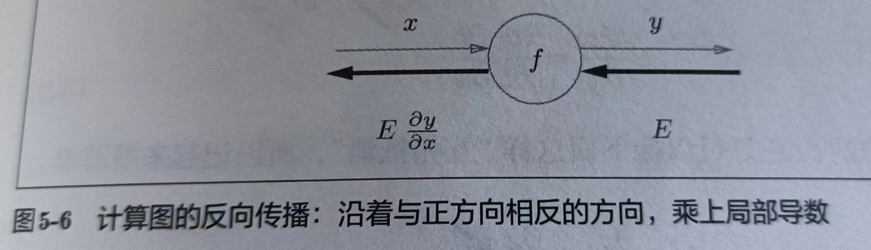
反向传播的计算顺序为,将信号E乘以结点的局部导数,然后将结果传递给下一个结点
5.3 反向传播
5.3.1 加法层的实现
p130
加法节点的反向传播只乘以1,所以输入的值会原封不动地流向下一个节点。
比如z(x,y) = x+y,求x和y求导都是1
5.4 简单层的实现
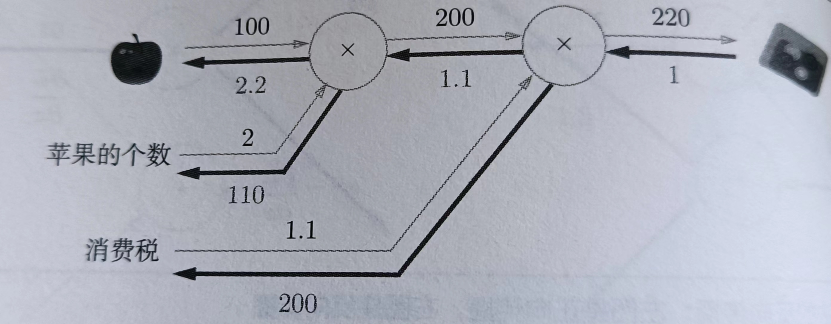
5.4.1 乘法层的实现
p135
class MulLayer:
    def __init__(self):
        self.x = None
        self.y = None

    def forward(self,x,y):
        self.x = x
        self.y = y
        out = x * y
        return out

    def backward(self,dout):
        dx = dout * self.y
        dy = dout * self.x

        return dx,dy

apple = 100
apple_num = 2
tax = 1.1

mul_apple_layer = MulLayer()
mul_tax_layer = MulLayer()

# forward
apple_price = mul_apple_layer.forward(apple,apple_num)
price = mul_tax_layer.forward(apple_price,tax)
print(price) # 220

# backward
dprice = 1
dapple_price,dtax = mul_tax_layer.backward(dprice)
dapple,dapple_num = mul_apple_layer.backward(dapple_price)
print(dapple_price,dtax,dapple,dapple_num) # 1.1 200 2.2 110
5.4.2 加法层的实现
p137
class AddLayer:
    def __init__(self):
        pass  # pass 表示什么也不运行

    def forward(self,x,y):
        out = x + y
        return out

    def backward(self,dout):
        dx = dout * 1
        dy = dout * 1
        return dx,dy
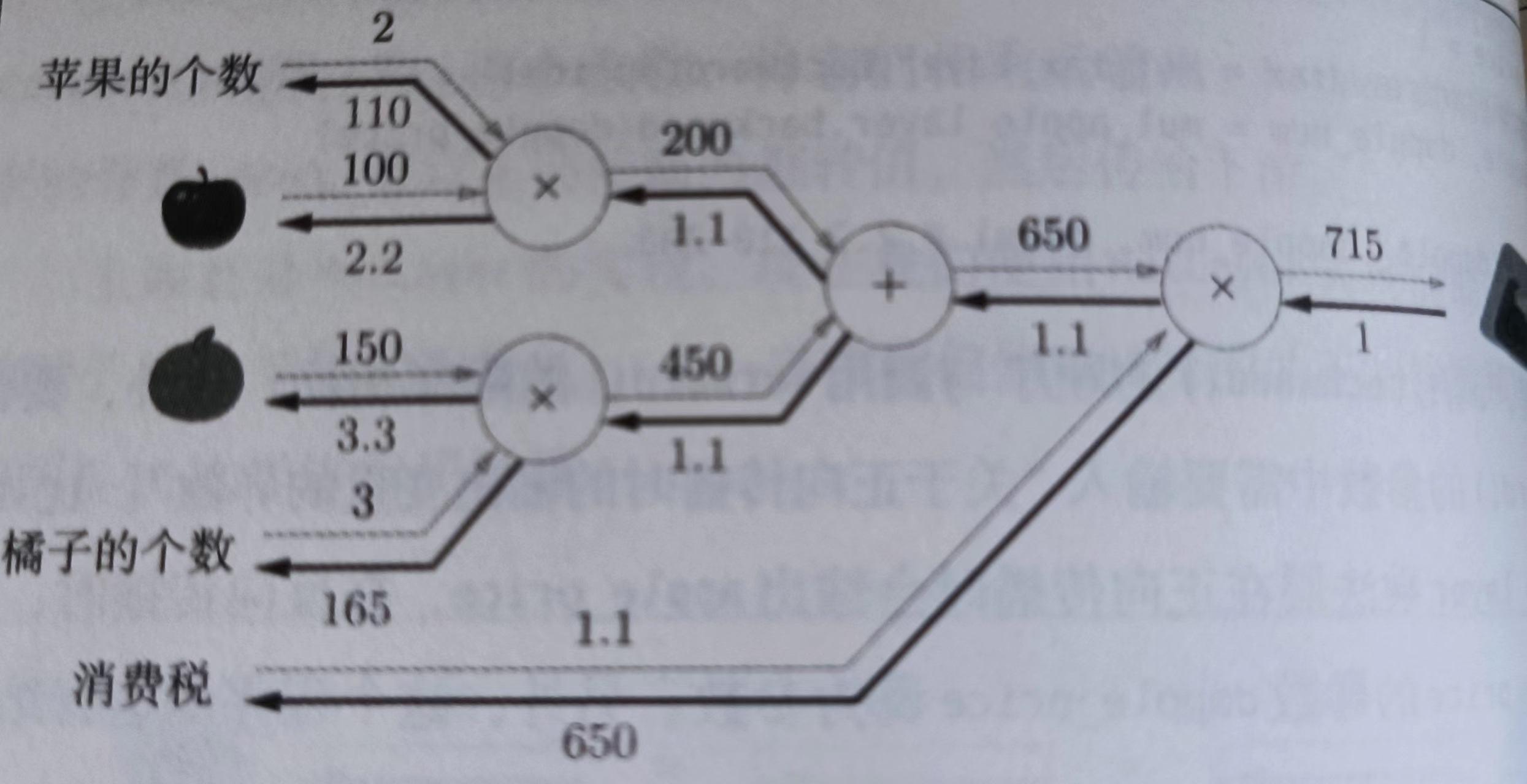
5.4.3 组合实现
p138
class AddLayer:
    def __init__(self):
        pass  # pass 表示什么也不运行

    def forward(self,x,y):
        out = x + y
        return out

    def backward(self,dout):
        dx = dout * 1
        dy = dout * 1
        return dx,dy

class MulLayer:
    def __init__(self):
        self.x = None
        self.y = None

    def forward(self,x,y):
        self.x = x
        self.y = y
        out = x * y
        return out

    def backward(self,dout):
        dx = dout * self.y
        dy = dout * self.x

        return dx,dy

apple = 100
apple_num = 2
orange = 150
orange_num = 3
tax = 1.1

# layer
mul_apple_layer = MulLayer()
mul_orange_layer = MulLayer()
add_apple_orange_layer = AddLayer()
mul_tax_layer = MulLayer()

# forward
apple_price = mul_apple_layer.forward(apple,apple_num)
orange_price = mul_orange_layer.forward(orange,orange_num)
all_price = add_apple_orange_layer.forward(apple_price,orange_price)
price = mul_tax_layer.forward(all_price,tax)

# backward
dprice = 1
dall_price,dtax = mul_tax_layer.backward(dprice)
dapple_price,dorange_price = add_apple_orange_layer.backward(dall_price)
dorange,dorange_num = mul_orange_layer.backward(dorange_price)
dapple,dapple_num = mul_apple_layer.backward(dapple_price)

print(price) # 715
print(dapple_num,dapple,dorange,dorange_num,dtax) # 110,2.2,3.3,165,650
5.5 激活函数层的实现
5.5.1 ReLu层的实现
p140
import numpy as np


class Relu:
    def __init__(self):
        self.mask = None

    def forward(self,x):
        self.mask  = (x <= 0)
        out = x.copy()
        out[self.mask] = 0

    def backward(self,dout):
        dout[self.mask] = 0
        dx = dout
        return dx

x = np.array([[1.0,-0.5],[-2.0,3.0]])
print(x)
# [[ 1.  -0.5]
#  [-2.   3. ]]

mask = (x <= 0)
print(mask)
# [[False  True]
#  [True   False]]
mask变量是由True/False组成的numpy数组,它会把正向传播中x中元素小于等于0的地方保存为True,其他地方保存为False。
如果正向传播的输入值小于等于0,则反向传播的值为0,因此,反向传播中会使用正向传播时保存的mask,将从上游传来的dout的mask中的元素为True的地方设为0
5.5.2 Sigmoid层
p141
sigmoid反向传播流程

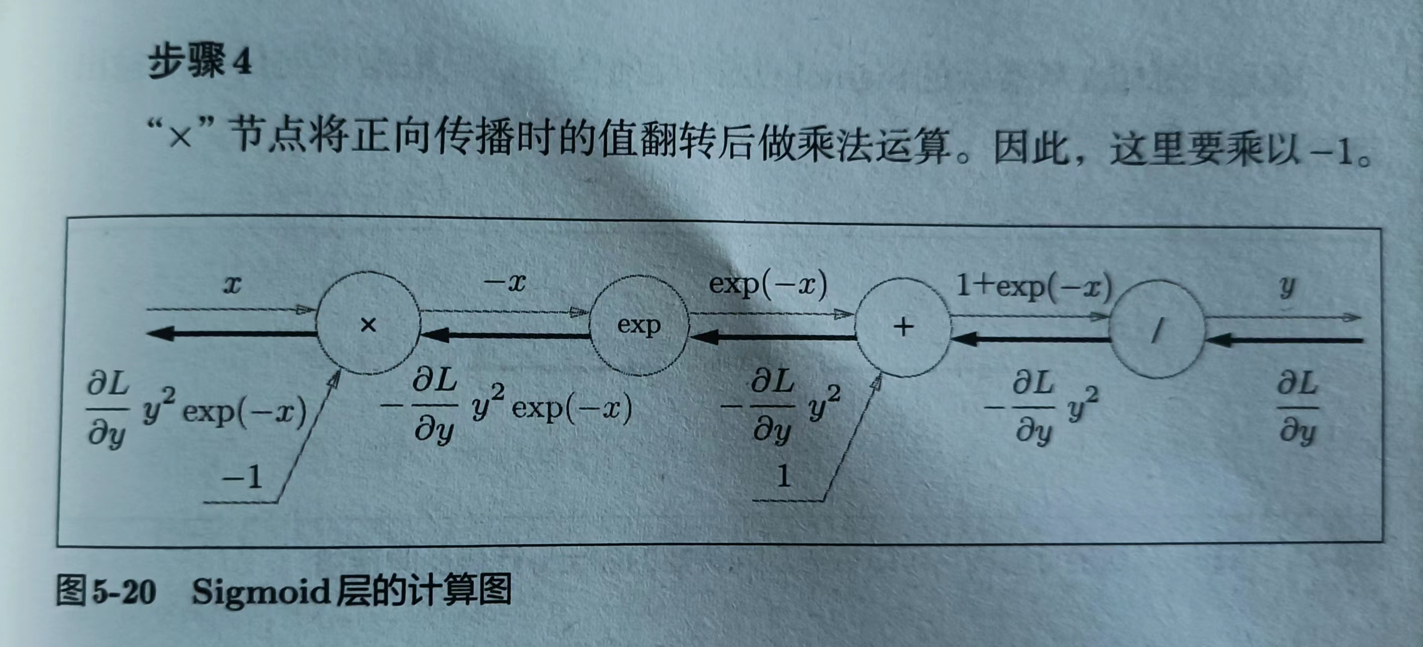
sigmoid层的计算图简洁版
简洁版效率更高,不用在意sigmoid层中的琐碎细节

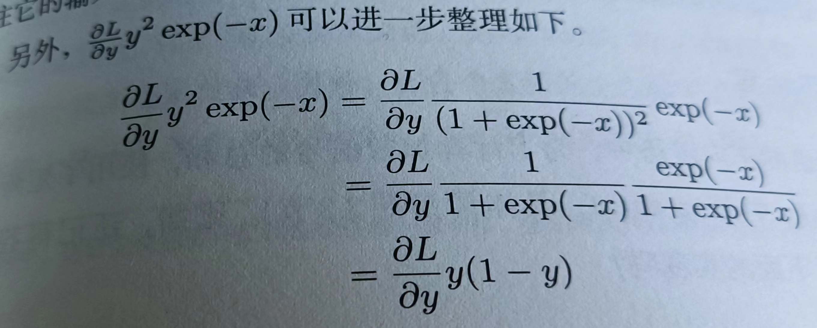
对公式进行整理
代码实现
import numpy as np

class Sigmoid:
    def __init__(self):
        self.out = None

    def forward(self,x):
        out = 1 / (1 + np.exp(-x))
        return out

    def backward(self,dout):
        dx = dout * (1.0 - self.out) * self.out
        return dx
5.6 Affine/Softmax层的实现
5.6.1 Affine层
p145
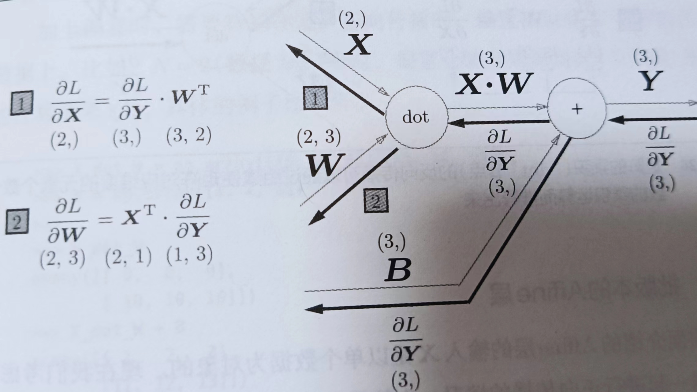
神经网络的正向传播中进行的矩阵的乘积运算在几何学领域被统称为“仿射变换”。这里将仿射变换的处理实现为“Affine层”
这里,X,W,B分别是形状为(2,),(2,3),(3,)的多维数组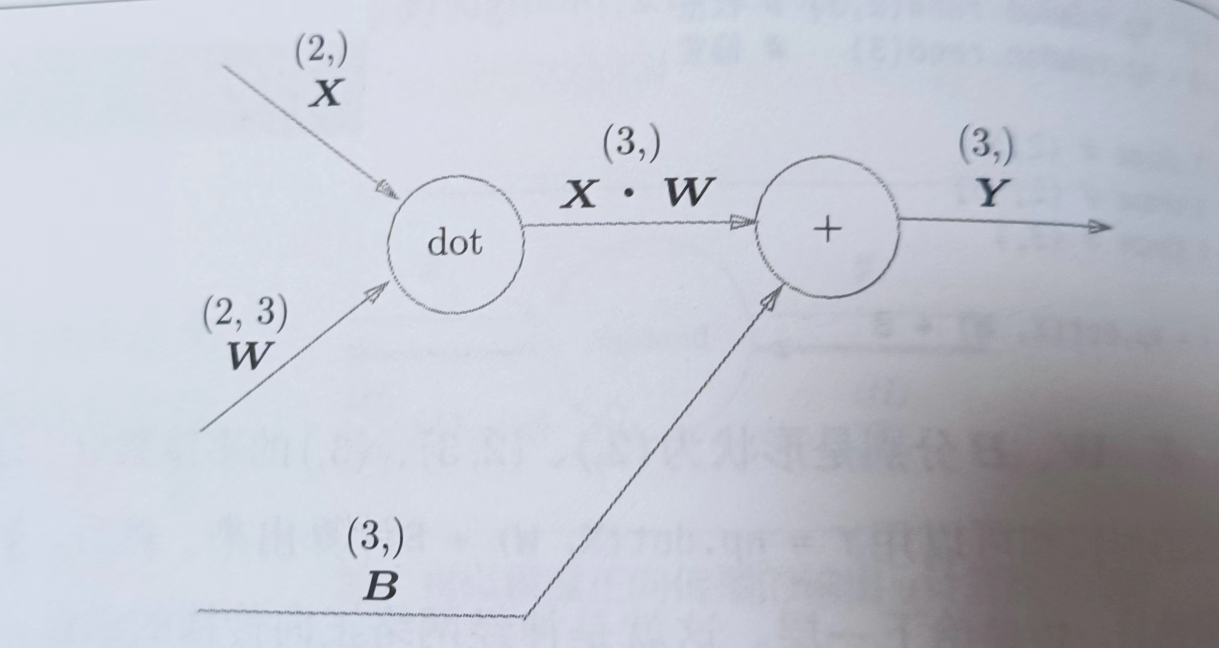
(X· W)+B后得到Y,Y的维度是(3,),Y求完导后还是(3,),反推得到下式
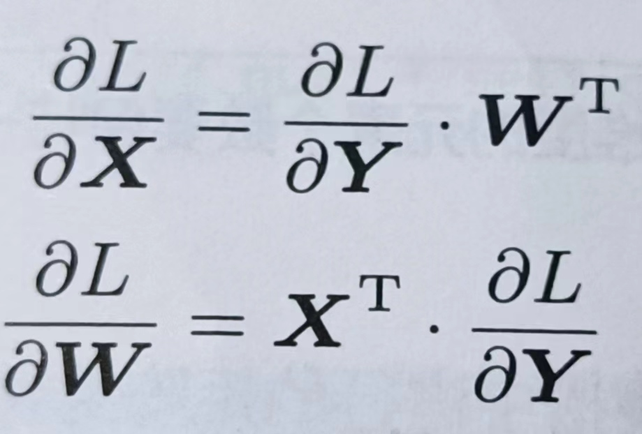
因为X维度是(2,),所以右边的式子的维度也要求是(2,),因此后面的式子那样写,只有那样它们相乘的维度才是(2,),这里的X是单个数据为对象的
5.6.2 批版本的Affine层
p148
上面的Affine层的X是单个数据为对象的。现在把N个数据一起进行正向传播的情况,也就是批版本的Affine层。
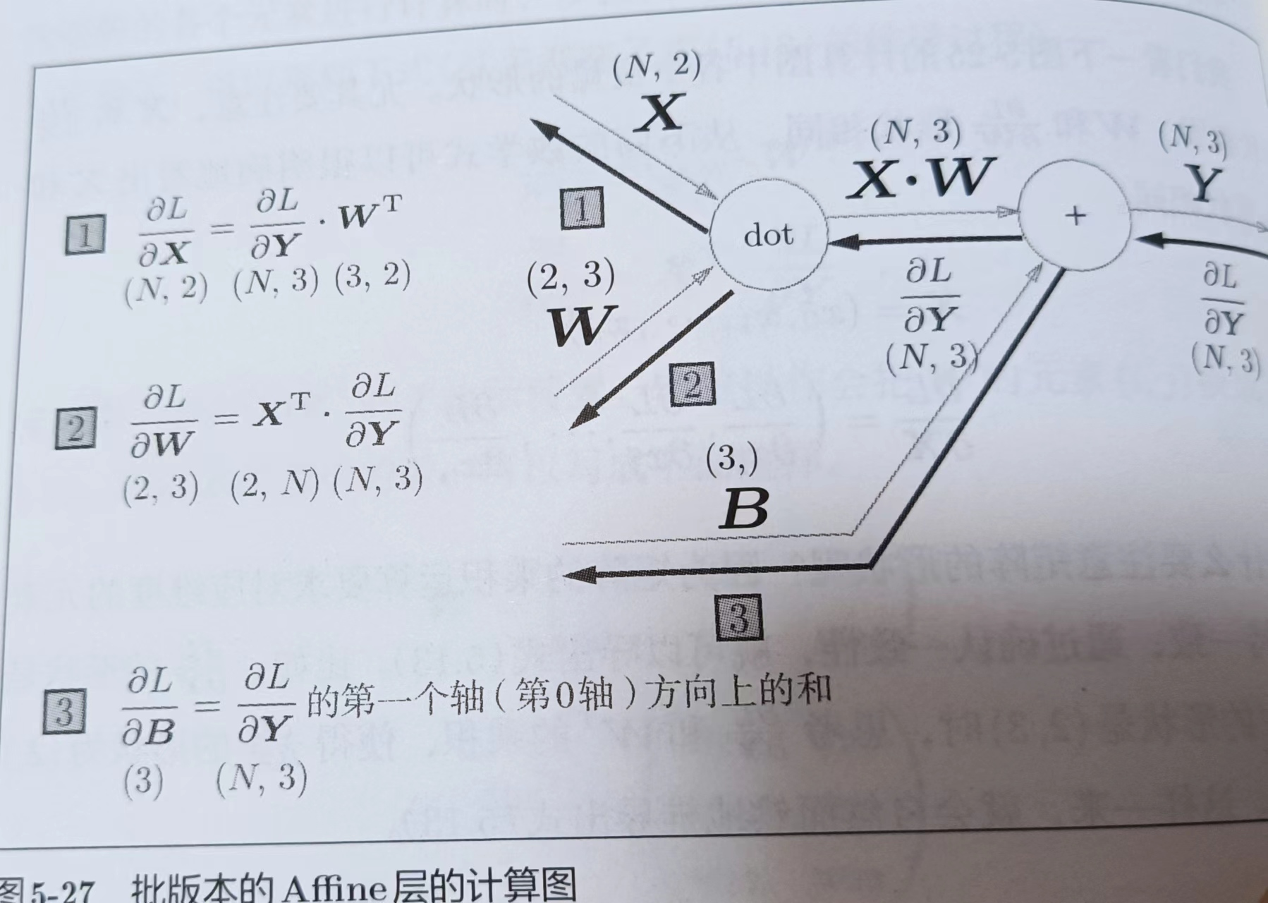
矩阵的形状
b里面有3个元素,所以维度是(3,),x_dot_w里面有2个数组,每个数组里面有3个元素,所以维度是(2,3),y里面有3个数组,每个数组里面又有2个数组,数组有4个元素,所以维度是(2,3,4)
b = np.array([1,2,3])
print(b.shape,np.ndim(b)) # (3,) 1

x_dot_w = np.array([[1,2,3],
              [4,5,6]])
print(x_dot_w.shape,np.ndim(x_dot_w)) # (2, 3) 2

y = np.array([
    [
        [1,2,3,0],
        [4,5,6,0]
    ],
    [
        [7,8,9,0],
        [10,11,12,0]
    ],
    [
        [17, 28, 29, 20],
        [210, 121, 122, 20]
    ]
])
print(y.shape,np.ndim(y)) # (3, 2, 4) 3
Affine层的实现
import numpy as np

class Affine:
    def __init__(self,W,b):
        self.W = W
        self.b = b
        self.x = None
        self.dW = None
        self.db = None

    def forward(self,x):
        self.x = x
        out = np.dot(x,self.W) + self.b
		return out

    def backward(self,dout):
        dx = np.dot(dout,self.W.T)
        self.dW = np.dot(self.x.T,dout)
        self.db = np.sum(dout,axis=0)

        return dx

b = np.array([[1,2,3],
              [4,5,6]])
print(b.T)
# [[1 4]
#  [2 5]
#  [3 6]]
5.6.3 softmax-with-loss层
p152
神经网络学习的目的就是通过调整权重参数,使神经网络的输出(softmax的输出)接近监督标签。因此,必须将神经网络的输出与监督标签的误差高效地传递给前面的层。使用交叉熵作为softmax函数的损失函数后,反向传播得到了(y1-t1,y2-t2,y3-t3),为了得到这样的结果特意设计交叉熵误差函数。回归问题中输出层使用恒等函数,损失函数使用"平方和误差"作为“恒等函数"的损失函数,反向传播也能得到(y1-t1,y2-t2,y3-t3)这样的结果
代码实现
import numpy as np

def softmax(x):
    if x.ndim == 2:
        x = x.T
        x = x - np.max(x, axis=0)
        y = np.exp(x) / np.sum(np.exp(x), axis=0)
        return y.T

    x = x - np.max(x)  # 溢出对策
    return np.exp(x) / np.sum(np.exp(x))

def cross_entropy_error(y, t):
    if y.ndim == 1:
        t = t.reshape(1, t.size)
        y = y.reshape(1, y.size)

    # 监督数据是one-hot-vector的情况下,转换为正确解标签的索引
    if t.size == y.size:
        t = t.argmax(axis=1)

    batch_size = y.shape[0]
    return -np.sum(np.log(y[np.arange(batch_size), t] + 1e-7)) / batch_size

class SoftmaxWithLoss:
    def __init__(self):
        self.loss = None   # 损失
        self.y = None # softmax的输出
        self.t = None # 监督数据(one-hot vector)

    def forward(self,x,t):
        self.t = t
        self.y = softmax(x)
        self.loss = cross_entropy_error(self.y,self.t)

        return self.loss

    def backward(self,dout=1):
        batch_size = self.t.shape[0]
        dx = (self.y - self.t) / batch_size

        return dx
反向传播时,将要传输的值除以批次大小,传递给前面的是单个数据的误差
5.7 误差反向传播法的实现
5.7.2 对应误差反向传播法的神经网络的实现
p156
import sys,os
sys.path.append(os.pardir)
import numpy as np
from common.layers import *
from common.gradient import numerical_gradient
from collections import OrderedDict

class TwoLayerNet:
    def __init__(self,input_size,hidden_size,output_size,weight_init_std=0.01):
        # 初始化权重
        self.params = {}
        self.params['W1'] = weight_init_std * np.random.randn(input_size,hidden_size)
        self.params['b1'] = np.zeros(hidden_size)
        self.params['W2'] = weight_init_std * np.random.randn(hidden_size,output_size)
        self.params['b2'] = np.zeros(output_size)

        # 生成层
        self.layers = OrderedDict() # 让字典有序
        self.layers['Affine1'] = Affine(self.params['W1'],self.params['b1'])
        self.layers['Relu1'] = Relu()
        self.layers['Affine2'] = Affine(self.params['W2'],self.params['b2'])
        self.lastLayer = SoftmaxWithLoss()

    def predict(self,x):
        for layer in self.layers.values():
            x = layer.forward(x)

        return x

    # x:输入数据,t:监督数据
    def loss(self,x,t):
        y = self.predict(x)
        return self.lastLayer.forward(y,t)

    def accuracy(self,x,t):
        y = self.predict(x)
        y = np.argmax(y,axis=1)
        if t.ndim != 1 : t = np.argmax(t,axis=1)
        accuracy = np.sum(y == t) / float(x.shape[0])
        return accuracy

    # x:输入数据,t:监督数据
    def numerical_gradient(self,x,t):
        loss_W = lambda W:self.loss(x,t)

        grads = {}
        grads['W1'] = numerical_gradient(loss_W,self.params['W1'])
        grads['b1'] = numerical_gradient(loss_W,self.params['b1'])
        grads['W2'] = numerical_gradient(loss_W,self.params['W2'])
        grads['b2'] = numerical_gradient(loss_W,self.params['b2'])

        return grads

    def gradient(self,x,t):
        # forward
        self.loss(x,t)

        # backward
        dout = 1
        dout = self.lastLayer.backward(dout)

        layers = list(self.layers.values())
        layers.reverse() # 反转
        for layer in layers:
            dout = layer.backward(dout)

        # 设定
        grads = {}
        grads['W1'] = self.layers['Affine1'].dW
        grads['b1'] = self.layers['Affine1'].db
        grads['W2'] = self.layers['Affine2'].dW
        grads['b2'] = self.layers['Affine2'].db

        return grads
5.7.3 误差反向传播法的梯度确认
这里有两种求梯度的方法
- 基于数值微分,实现简单,不太容易出错,但是很耗费时间
- 解析性地求解数学式的方法(误差反向传播法),即使存在大量参数,也可以高效计算梯度,但是实现复杂,容易出错
在确认误差反向传播法的实现是否正确时,是需要用到数值微分的。所以,经常会比较数值微分的结果和误差反向传播法的结果,确认误差反向传播的实现是否正确。
梯度确认是值确认数值微分和误差反向传播法的实现是否一致(严格说,是非常相近)
p158
import sys,os
sys.path.append(os.pardir)
import numpy as np
from dataset.mnist import load_mnist
from twolayernet import TwoLayerNet

# 读入数据
(x_train,t_train),(x_test,t_test) = load_mnist(normalize=True,one_hot_label=True)

network = TwoLayerNet(input_size=784,hidden_size=50,output_size=10)

x_batch = x_train[:3]
t_batch = t_train[:3]

grad_numerical = network.numerical_gradient(x_batch,t_batch)
grad_backprop = network.gradient(x_batch,t_batch)

# 求各个权重的绝对值误差的平均值
for key in grad_numerical.keys():
    diff = np.average(np.abs(grad_backprop[key] - grad_numerical[key]))
    print(key + ":"+str(diff))
5.7.4 误差反向传播法的学习
p160
import sys,os
sys.path.append(os.pardir)
import numpy as np
from dataset.mnist import load_mnist
from twolayernet import TwoLayerNet

# 读入数据
(x_train,t_train),(x_test,t_test) = load_mnist(normalize=True,one_hot_label=True)

network = TwoLayerNet(input_size=784,hidden_size=50,output_size=10)

# 设置超参数
iters_num = 10000
train_size = x_train.shape[0]
batch_size = 100
learning_rate = 0.1
train_loss_list = []
train_acc_list = []
test_acc_list = []

iter_per_epoch = max(train_size / batch_size,1)

for i in range(iters_num):
    batch_mask = np.random.choice(train_size,batch_size)
    x_batch = x_train[batch_mask]
    t_batch = t_train[batch_mask]

    # 通过误差反向传播法求梯度
    grad = network.gradient(x_batch,t_batch)

    # 更新
    for key in ('W1','b1','W2','b2'):
        network.params[key] -= learning_rate * grad[key]

    loss = network.loss(x_batch,t_batch)
    train_loss_list.append(loss)

    if i % iter_per_epoch == 0:
        train_acc = network.accuracy(x_train,t_train)
        test_acc = network.accuracy(x_test,t_test)
        train_acc_list.append(train_acc)
        test_acc_list.append(test_acc)
        print(train_acc,test_acc)
第6章 与学习相关的技巧
6.1 参数的更新
6.1.2 SGD
SGD低效的根本原因是梯度的方向没有指向最小值的方向
p165
class SGD:
    def __init__(self,lr=0.01):
        self.lr = lr

    def update(self,params,grads):
        for key in params.keys():
            params[key] -= self.lr * grads[key]
6.1.4 Momentum(冲量)
p168
公式如下
αv:该项承担使物体逐渐减速的任务,对应的是物理中的地面摩擦力或空气阻力
代码实现
import numpy as np


class Momentum:
    def __init__(self,lr=0.01,momentum=0.9):
        self.lr = lr
        self.momentum = momentum
        self.v = None

    def update(self,params,grads):
        if self.v is None:
            self.v = {}
            for key, val in params.items():
                self.v[key] = np.zeros_like(val)

        for key in params.keys():
            self.v[key] = self.momentum*self.v[key] - self.lr * grads[key]
            params[key] += self.v[key]
v保存物体的速度,初始化时,v中什么都不保存,但当第一次调用update()时,v会以字典变量的形式保存与参数结构相同的数据
6.1.5 AdaGrad
p170
AdaGrad会为参数的每个元素适当地调节学习率,它会记录过去所有梯度的平方和,因此,学习越深入,更新的幅度越小。如果无止境的学习,更新量就会为0,完全不再更新。RMSProp可以改善这个问题,它会逐渐忘掉过去的梯度。
公式如下
这里的h它保存了以前的所有梯度的平方和。可以使变动大的元素的学习率变小,使变动小的元素的学习率变大。
代码实现
import numpy as np


class AdaGrad:
    def __init__(self,lr=0.01):
        self.lr = lr
        self.h = None

    def update(self,params,grads):
        if self.h is None:
            self.h = {}
            for key,val in params.items():
                self.h[key] = np.zeros_like(val)

        for key in params.keys():
            self.h[key] += grads[key] * grads[key]
            params[key] -= self.lr * grads[key] / (np.sqrt(self.h[key]) + 1e-7)
6.1.6 Adam
p173
Adam通俗来讲,就是融合了Momentum和AdaGrad的方法
6.2 权重的初始值
6.2.1 可以将权重初始值设为0吗
p176
不可以,权重设置为0,严格来说,不能将权重设置为一样的值,因为权重被更新为相同的值,并拥有了对称的值(重复的值),使得神经网络拥有许多不同的权重的意义丧失了。因此,必须随机生成初始化值。
6.2.2 隐藏层的激活值的分布
p177
import numpy as np
import matplotlib.pyplot as plt

def sigmoid(x):
    return 1/(1+np.exp(-x))

x = np.random.randn(1000,100) # 1000×100的矩阵
node_num = 100 # 各隐藏层的节点(神经元)数
hidden_layer_size = 5 # 隐藏层有5层
activations = {}  # 激活值的结果保存在这里

for i in range(hidden_layer_size):
    if i!= 0:
        x = activations[i-1]

    # w = np.random.randn(node_num,node_num) * 1   # 使用标准差为1的高斯分布
    w = np.random.randn(node_num,node_num) * 0.01  # 使用标准差为0.01的高斯分布
    z = np.dot(x,w)
    a = sigmoid(z)
    activations[i] = a

# 绘制直方图
for i,a in activations.items():
    plt.subplot(1,len(activations),i+1)
    plt.title(str(i+1)+"-layer")
    plt.hist(a.flatten(),30,range=(0,1))
plt.show()
输出结果
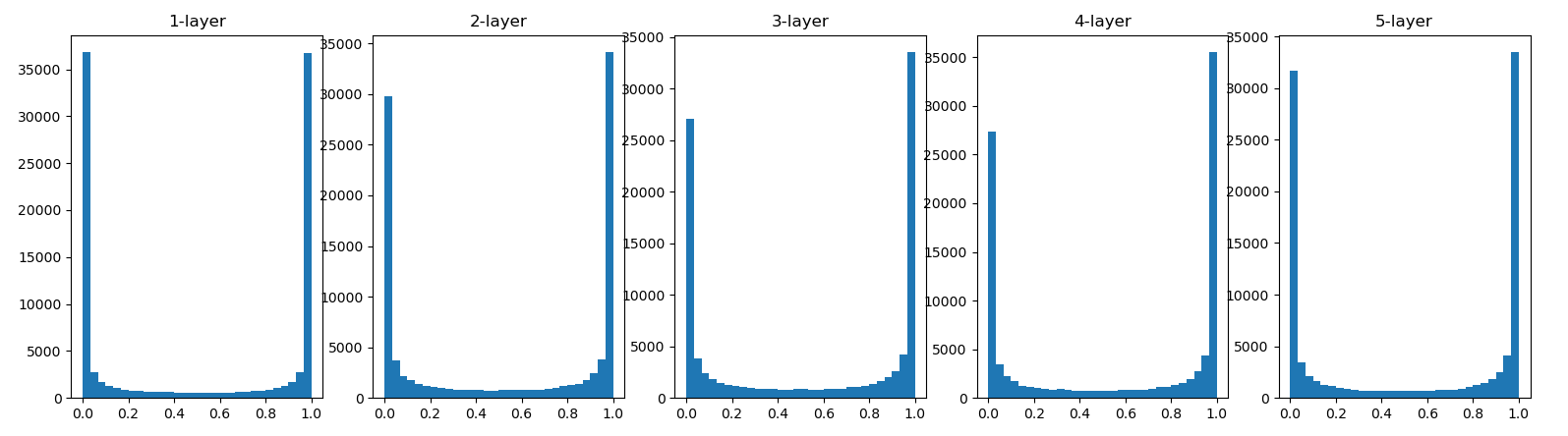
由上图可以知道,各层的激活值偏向0和1的分布,输出不断地靠近0或者1它的导数值逐渐接近0,。偏向0和1的数据分布,会造成反向传播中梯度的值不断减少,直至消失。这个问题称为梯度消失。
使用标准差为0.01的高斯分布如下图所示
w = np.random.randn(node_num,node_num) * 0.01
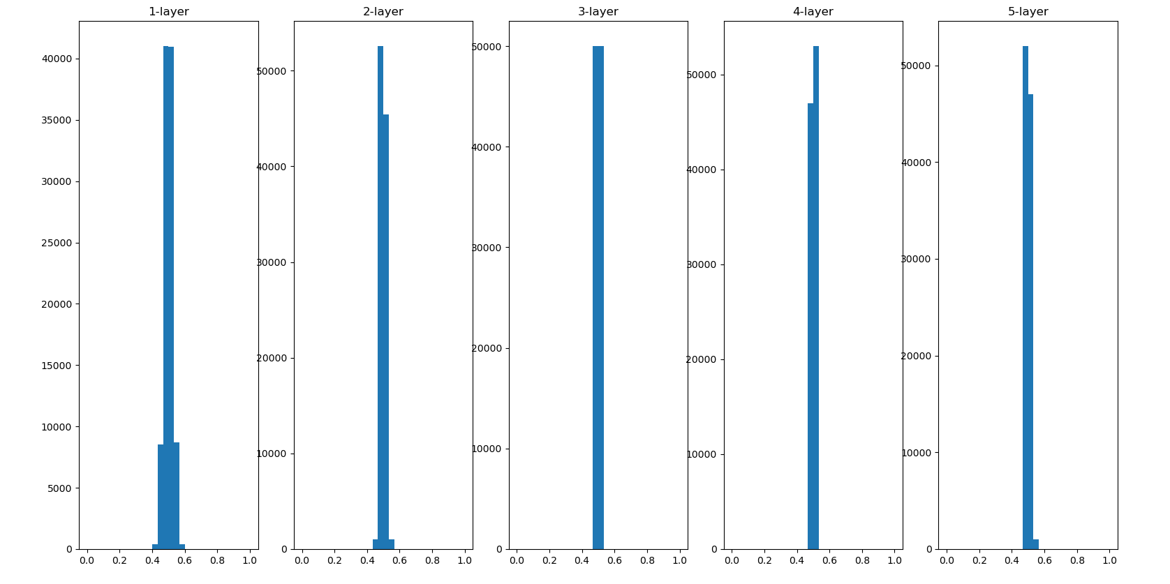
这次集中在0.5附近,不会有梯度消失的问题,但是这里的值都集中在0.5附近,会出现“表现力受限”的问题。
使用标准差为的高斯分布如下图所示
w = np.random.randn(node_num, node_num) / np.sqrt(node_num)
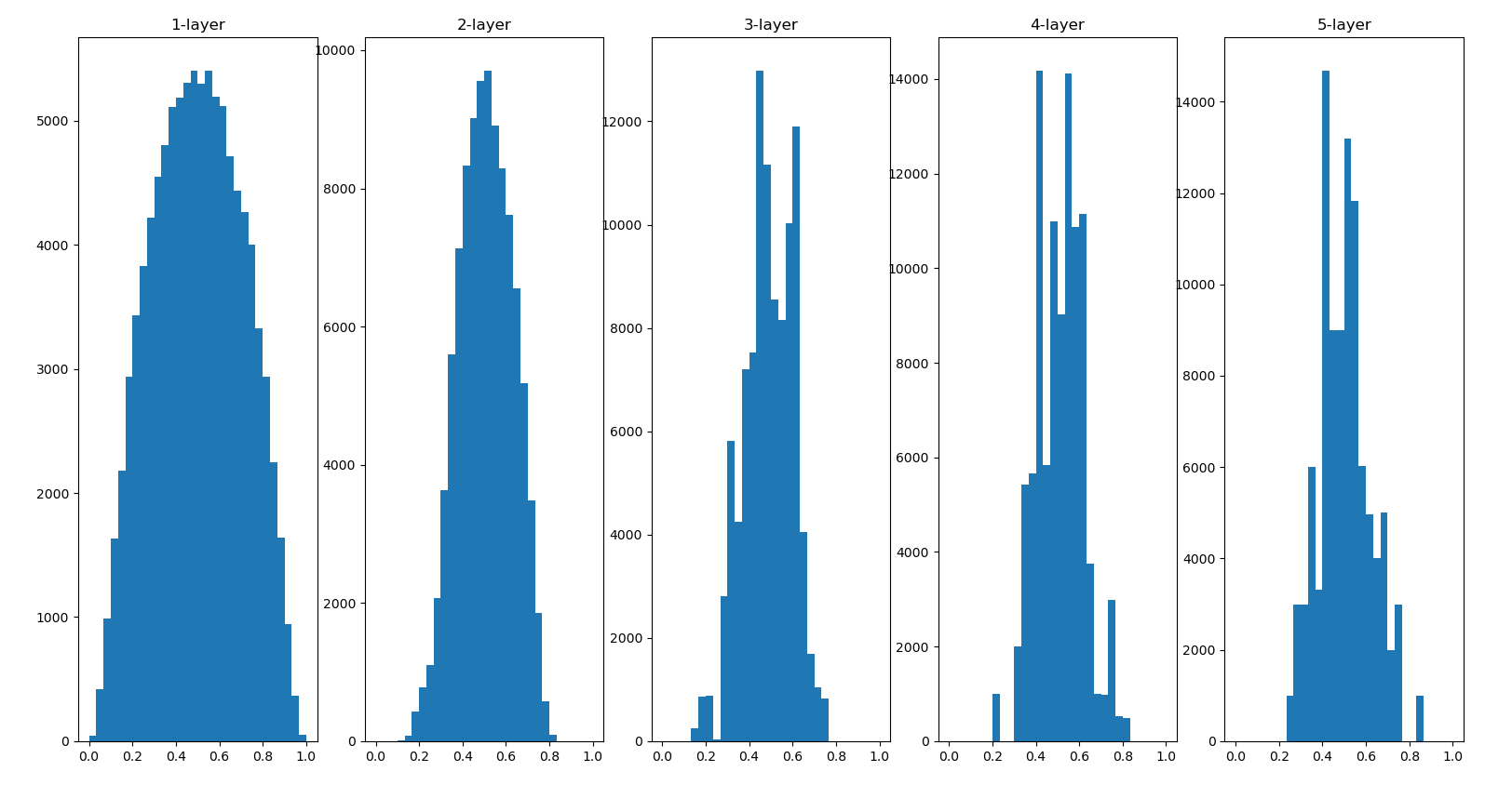
使用Xavier初始值(标准差为)后,比之前更有广度的分布,所以这里sigmoid函数的表现力不受限制。这里sigmoid换成tanh函数也可以。
当激活函数使用ReLU时,权重初始值使用He初始值(标准差为),激活函数是sigmoid或tanh等S型曲线函数时使用Xavier初始值。
6.3 Batch Normalization
p184
- 可以使学习快速进行(可以增大学习率)
- 不那么依赖初始值
- 抑制过拟合
6.4 正则化
6.4.1 过拟合
p189
过拟合的主要原因
- 模型拥有大量的参数,表现力强
- 训练数据小
6.4.2 权值衰减
p191
权值衰减可以用来抑制过拟合,在学习的过程中对大的权重进行惩罚,来抑制过拟合,很大过拟合是因为权重参数取值过大才发生的。让损失函数加上下面的任一一个正则化项
正则化项
- L1范数是各元素的绝对值之和
- L2范数是各个元素的平方和
- L∞范数是各个元素的绝对值中最大的那一个
6.4.3 Dropout
p193
一种抑制过拟合的方法,会在学习过程中随机删除神经元
import numpy as np


class Dropout:
    def __init__(self,dropout_ratio=0.5):
        self.dropout_ratio = dropout_ratio
        self.mask = None

    def forward(self,x,train_flg=True):
        if train_flg:
            self.mask = np.random.rand(*x.shape) > self.dropout_ratio
            print(self.mask)
            # [[True False]
            #  [True  True]]
            return x * self.mask

        else:
            return x * (1.0 - self.dropout_ratio)

    def backward(self,dout):
        return dout * self.mask

d = Dropout()
x = np.array([[1.0,-0.5],[-2.0,3.0]])
print(d.forward(x))
# [[ 1. -0.]
#  [-2.  3.]]
print(d.backward(1))
# [[1 0]
#  [1 1]]
*的作用:在函数定义中,收集所有位置参数到一个新的元组,并将整个元组赋值给变量
import numpy as np
x = np.array([[1,2],
              [3,4]])
print(np.random.rand(*x.shape))
# [[0.52955823 0.80267996]
#  [0.03912289 0.12095148]]
6.5 超参数的验证
超参数一般为神经元数量,batch大小,学习率,权值衰减等,不能使用测试数据评估超参数的性能,如果用测试数据确认超参数的好坏,会导致模型不能拟合其他数据,泛化能力低。
6.5.1 验证数据
p195
调整超参数时,必须用验证数据来评估超参数的好坏。训练数据用于参数(权重和偏置)的学习,验证数据用于超参数的性能评估,确认泛化能力,需要使用测试数据(最好只用一次)
一般拿到数据集后,会分成训练数据,验证数据,测试数据。如果数据集没有划分,需要自己手动划分,这里以MNIST为例,划分20%为验证数据。
(x_train,t_train),(x_test,t_test) = load_minist()

# 打乱训练数据
x_train,t_train = shuffle_dataset(x_train,t_train)

# 分割验证数据
validation_rate = 0.20
validation_num = int(x_train.shape[0]*validation_rate)

x_val = x_train[:validation_num]
t_val = t_train[:validation_num]
x_train = x_train[validation_num:]
t_train = t_train[validation_num:]
6.5.2 超参数的最优化
p197
步骤0
设定超参数的范围
步骤1
从设定的超参数范围中随机采样
步骤2
使用步骤1中采样的超参数的值进行学习,通过验证数据评估估计精度(但是要将epoch设置得很小)
步骤3
重复步骤1和步骤2(100次等),根据它们的识别精度的结果,缩小超参数的范围。
本文作者:放学别跑啊
本文链接:https://www.cnblogs.com/bzwww/p/16815910.html
版权声明:本作品采用知识共享署名-非商业性使用-禁止演绎 2.5 中国大陆许可协议进行许可。


【推荐】国内首个AI IDE,深度理解中文开发场景,立即下载体验Trae
【推荐】编程新体验,更懂你的AI,立即体验豆包MarsCode编程助手
【推荐】抖音旗下AI助手豆包,你的智能百科全书,全免费不限次数
【推荐】轻量又高性能的 SSH 工具 IShell:AI 加持,快人一步