LSTM情感分析
我们将导入两个不同的数据结构,一个是包含40000个单词的 Python列表,一个是包含所有单词向量值得400000*50维的嵌入矩阵。
import numpy as np
wordsList = np.load('./数据集/LSTM情感分析/training_data/wordsList.npy')# 包含40000个单词的 Python列表
print('Loaded the word List!')
print(type(wordsList)) # numpy.ndarray
wordsList = wordsList.tolist()
wordsList = [word.decode('UTF-8') for word in wordsList]
wordVectors = np.load('./数据集/LSTM情感分析/training_data/wordVectors.npy')#包含所有单词向量值得400000*50维的嵌入矩阵
print('Loaded the word vectors!')
print(len(wordsList))
print(wordVectors.shape)
Loaded the word List!
<class 'numpy.ndarray'>
Loaded the word vectors!
400000
(400000, 50)
我可以查看在词库中搜索“good",然后得到的index通过嵌入矩阵得到相应的向量
goodIndex = wordsList.index('good')
print(goodIndex) # 219
wordVectors[goodIndex]
array([-3.5586e-01,  5.2130e-01, -6.1070e-01, -3.0131e-01,  9.4862e-01,
       -3.1539e-01, -5.9831e-01,  1.2188e-01, -3.1943e-02,  5.5695e-01,
       -1.0621e-01,  6.3399e-01, -4.7340e-01, -7.5895e-02,  3.8247e-01,
        8.1569e-02,  8.2214e-01,  2.2220e-01, -8.3764e-03, -7.6620e-01,
       -5.6253e-01,  6.1759e-01,  2.0292e-01, -4.8598e-02,  8.7815e-01,
       -1.6549e+00, -7.7418e-01,  1.5435e-01,  9.4823e-01, -3.9520e-01,
        3.7302e+00,  8.2855e-01, -1.4104e-01,  1.6395e-02,  2.1115e-01,
       -3.6085e-02, -1.5587e-01,  8.6583e-01,  2.6309e-01, -7.1015e-01,
       -3.6770e-02,  1.8282e-03, -1.7704e-01,  2.7032e-01,  1.1026e-01,
        1.4133e-01, -5.7322e-02,  2.7207e-01,  3.1305e-01,  9.2771e-01],
      dtype=float32)
现在我们有了向量,我们的第一步就是输入一个句子,然后构造它的向量表示。假设我们现在的输入句子是 “I thought the movie was incredible and inspiring”。为了得到词向量,我们可以使用 TensorFlow 的嵌入函数。这个函数有两个参数,一个是嵌入矩阵(在我们的情况下是词向量矩阵),另一个是每个词对应的索引。
# 我这里tensorflow版本是2
import tensorflow as tf
maxSeqLength = 10 # 设置最大词数
numDimensions = 300 # 设置每个单词最大纬度
firstSentence = np.zeros((maxSeqLength),dtype='int32')
firstSentence
firstSentence[0] = wordsList.index('i')
firstSentence[1] = wordsList.index('thought')
firstSentence[2] = wordsList.index('the')
firstSentence[3] = wordsList.index('movie')
firstSentence[4] = wordsList.index('was')
firstSentence[5] = wordsList.index('incredible')
firstSentence[6] = wordsList.index('and')
firstSentence[7] = wordsList.index('inspiring')
# 如果长度没有达到设置标准,用0来占位
print(firstSentence.shape)
(10,)
# 查看索引
print(firstSentence)
[ 41 804 201534 1005 15 7446 5 13767 0 0]
数据管道如下图所示
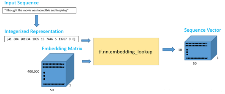
输出数据是一个 10*50 的词矩阵,其中包括 10 个词,每个词的向量维度是 50。就是去找到这些词对应的向量
tf.nn.embedding_lookup函数原理? - 知乎 (zhihu.com)
(20条消息) TensorFlow(九)eval函数_呆呆的猫的博客-CSDN博客_eval函数
with tf.compat.v1.Session() as sess:print(tf.nn.embedding_lookup(wordVectors,firstSentence).eval().shape)
(10, 50)
在整个训练集上面构造索引之前,我们先花一些时间来可视化我们所拥有的数据类型。这将帮助我们去决定如何设置最大序列长度的最佳值。在前面的例子中,我们设置了最大长度为 10,但这个值在很大程度上取决于你输入的数据。
训练集我们使用的是 IMDB 数据集。这个数据集包含 25000 条电影数据,其中 12500 条正向数据,12500 条负向数据。这些数据都是存储在一个文本文件中,首先我们需要做的就是去解析这个文件。正向数据包含在一个文件中,负向数据包含在另一个文件中。
Python os.listdir() 方法 | 菜鸟教程 (runoob.com)
Python os.path.isfile()用法及代码示例 - 纯净天空 (vimsky.com)
【Python】os.path.isfile()的使用方法汇总 - iSZ - 博客园 (cnblogs.com)
from os import listdir
from os.path import isfile,join

# 使用列表生成式,生成每一个普通文件的路径
positiveFiles = ['./数据集/LSTM情感分析/training_data/positiveReviews/'+ f for f in listdir('./数据集/LSTM情感分析/training_data/positiveReviews/') if isfile(join('./数据集/LSTM情感分析/training_data/positiveReviews/',f))]

negativeFiles = ['./数据集/LSTM情感分析/training_data/negativeReviews/'+ f for f in listdir('./数据集/LSTM情感分析/training_data/negativeReviews/') if isfile(join('./数据集/LSTM情感分析/training_data/negativeReviews/',f))]

numWords = []

# 将每个文件的每一行的单词数记录下来
for pf in positiveFiles:
    with open(pf,"r",encoding='utf-8') as f:
        line = f.readline()
        counter = len(line.split())
        numWords.append(counter)
print('Positive files finished')


for nf in negativeFiles:
    with open(nf,"r",encoding='utf-8') as f:
        line = f.readline()
        counter = len(line.split())
        numWords.append(counter)
print('Negative files finished')

numFiles = len(numWords)
print('The total number of files is', numFiles)
print('The total number of words in the files is', sum(numWords))
print('The average number of words in the files is', sum(numWords)/len(numWords))
Positive files finished
Negative files finished
The total number of files is 25000
The total number of words in the files is 5844680
The average number of words in the files is 233.7872
绘制直方图,来查看每行单词数的频率
import matplotlib.pyplot as plt
%matplotlib inline
plt.hist(numWords,50) # 这个50是直方图的柱数,即分组个数
plt.xlabel('Sequence Length')
plt.ylabel('Frequency')
plt.axis([0,1200,0,8000])
plt.show()
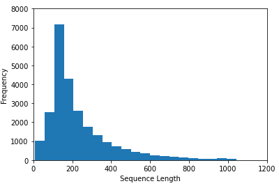
从直方图和句子的平均单词数,我们认为将句子最大长度设置为绝大多数的长度 250 是可行的。
maxSeqLength = 250

# 查看其中一条评论
fname = positiveFiles[3]
with open(fname) as f:
    for lines in f:
        print(lines)
        exit
接下来,我们将它转换成一个索引矩阵。
# 删除标点符号、括号、问号等,只留下字母数字字符
import re
strip_special_chars = re.compile("[^A-Za-z0-9 ]+")

def cleanSentences(string):
    string = string.lower().replace("<br />", "")
    return re.sub(strip_special_chars,"",string.lower())
firstFile = np.zeros((maxSeqLength),dtype='int32')
with open(fname) as f:
    indexCounter = 0
    line = f.readline()
    cleanedLine = cleanSentences(line)
    split = cleanedLine.split()
    # 把每一个单词在wordlist里面的索引存到firstFile里面
    for word in split:
        try:
            firstFile[indexCounter] = wordsList.index(word)
        except ValueError:
            firstFile[indexCounter] = 399999 # vector for unknown words
        indexCounter = indexCounter + 1
firstFile
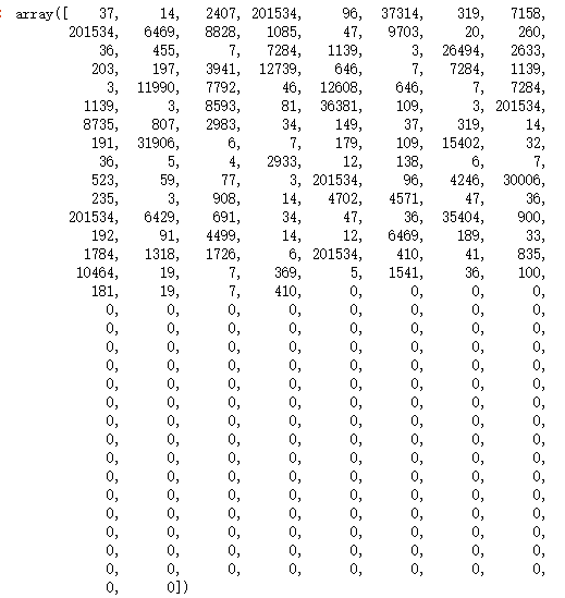
现在,我们用相同的方法来处理全部的 25000 条评论。我们将导入电影训练集,并且得到一个 25000 * 250 的矩阵。这是一个计算成本非常高的过程,可以直接使用理好的索引矩阵文件。
ids = np.load('./数据集/LSTM情感分析/training_data/idsMatrix.npy')
构建LSTM网络模型
RNN Model
现在,我们可以开始构建我们的 TensorFlow 图模型。首先,我们需要去定义一些超参数,比如批处理大小,LSTM的单元个数,分类类别和训练次数。
batchSize = 24  # 梯度处理的大小
lstmUnits = 64  # 隐藏层神经元数量
numClasses = 2  # 分类数量,n/p
iterations = 50000  # 迭代次数
与大多数 TensorFlow 图一样,现在我们需要指定两个占位符,一个用于数据输入,另一个用于标签数据。对于占位符,最重要的一点就是确定好维度。
标签占位符代表一组值,每一个值都为 [1,0] 或者 [0,1],这个取决于数据是正向的还是负向的。输入占位符,是一个整数化的索引数组。
(20条消息) tf.placeholder使用说明_陈 超的博客-CSDN博客_tf.placeholder()
tf.compat.v1.reset_default_graph()

tf.compat.v1.disable_eager_execution() # 不加这句话下面代码会报错

labels = tf.compat.v1.placeholder(tf.float32,[batchSize,numClasses])
input_data = tf.compat.v1.placeholder(tf.int32,[batchSize,maxSeqLength])
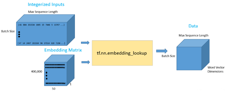
一旦,我们设置了我们的输入数据占位符,我们可以调用 tf. nn. embedding lookup0函数来得到我们的词向量。该函数最后将返回一个三维向量,第一个维度是批处理大小,第二个维度是句子长度,第三个维度是词向量长度。
(20条消息) TensorFlow图变量tf.Variable的用法解析_烧煤的快感的博客-CSDN博客_tf.variable
data = tf.Variable(tf.zeros([batchSize,maxSeqLength,numDimensions]),dtype = tf.float32)
data = tf.nn.embedding_lookup(wordVectors,input_data)
现在我们已经得到了我们想要的数据形式,那么揭晓了我们看看如何才能将这种数据形式输入到我们的 LSTM 网络中。首先,我们使用 tf.nn.rnn_cell.BasicLSTMCell 函数,这个函数输入的参数是一个整数,表示需要几个 LSTM 单元。这是我们设置的一个超参数,我们需要对这个数值进行调试从而来找到最优的解。然后,我们会设置一个 dropout 参数,以此来避免一些过拟合。
最后,我们将 LSTM cell 和三维的数据输入到 tf.nn.dynamic_rnn ,这个函数的功能是展开整个网络,并且构建一整个 RNN 模型。
lstmCell = tf.compat.v1.nn.rnn_cell.BasicLSTMCell(lstmUnits) # 基本单元
lstmCell = tf.compat.v1.nn.rnn_cell.DropoutWrapper(cell=lstmCell,output_keep_prob=0.75) # 解决一些过拟合问题,output_keep_prob保留比例
value,_ = tf.compat.v1.nn.dynamic_rnn(lstmCell,data,dtype=tf.float32) # 构建网络,value是值h,_ 是中间传递结果,这里不需要分析所以去掉
可能会遇到的错误
tensoflow模型中提示:ValueError: Variable rnn/basic_rnn_cell/kernel already exists, disallowed. Did you mean to set reuse=True or reuse=tf.AUTO_REUSE in VarScope
堆栈 LSTM 网络是一个比较好的网络架构。也就是前一个LSTM 隐藏层的输出是下一个LSTM的输入。堆栈LSTM可以帮助模型记住更多的上下文信息,但是带来的弊端是训练参数会增加很多,模型的训练时间会很长,过拟合的几率也会增加。
dynamic RNN 函数的第一个输出可以被认为是最后的隐藏状态向量。这个向量将被重新确定维度,然后乘以最后的权重矩阵和一个偏置项来获得最终的输出值。
# 权重参数初始化
weight = tf.Variable(tf.compat.v1.random.truncated_normal([lstmUnits, numClasses]))
bias = tf.Variable(tf.constant(0.1, shape=[numClasses]))
value = tf.transpose(value, [1, 0, 2])
# 获取最终的结果值
last = tf.gather(value, int(value.get_shape()[0]) - 1)  # 去ht
prediction = (tf.matmul(last, weight) + bias)  # 最终连上w和b
接下来,我们需要定义正确的预测函数和正确率评估参数。正确的预测形式是查看最后输出的0-1向量是否和标记的0-1向量相同。
correctPred = tf.equal(tf.argmax(prediction,1), tf.argmax(labels,1))
accuracy = tf.reduce_mean(tf.cast(correctPred, tf.float32))
之后,我们使用一个标准的交叉熵损失函数来作为损失值。对于优化器,我们选择 Adam,并且采用默认的学习率
loss = tf.reduce_mean(tf.nn.softmax_cross_entropy_with_logits(logits=prediction, labels=labels))
optimizer = tf.compat.v1.train.AdamOptimizer().minimize(loss)
训练与测试结果
超参数调整
选择合适的超参数来训练你的神经网络是至关重要的。你会发现你的训练损失值与你选择的优化器(Adam,Adadelta,SGD,等等),学习率和网络架构都有很大的关系。特别是在RNN和LSTM中,单元数量和词向量的大小都是重要因素。
学习率:RNN最难的一点就是它的训练非常困难,因为时间步骤很长。那么,学习率就变得非常重要了。如果我们将学习率设置的很大,那么学习曲线就会波动性很大,如果我们将学习率设置的很小,那么训练过程就会非常缓慢。根据经验,将学习率默认设置为 0.001 是一个比较好的开始。如果训练的非常缓慢,那么你可以适当的增大这个值,如果训练过程非常的不稳定,那么你可以适当的减小这个值。
优化器:这个在研究中没有一个一致的选择,但是 Adam 优化器被广泛的使用。
LSTM单元的数量:这个值很大程度上取决于输入文本的平均长度。而更多的单元数量可以帮助模型存储更多的文本信息,当然模型的训练时间就会增加很多,并且计算成本会非常昂贵。
词向量维度:词向量的维度一般我们设置为50到300。维度越多意味着可以存储更多的单词信息,但是你需要付出的是更昂贵的计算成本。
训练
训练过程的基本思路是,我们首先先定义一个 TensorFlow 会话。然后,我们加载一批评论和对应的标签。接下来,我们调用会话的 run 函数。这个函数有两个参数,第一个参数被称为 fetches 参数,这个参数定义了我们感兴趣的值。我们希望通过我们的优化器来最小化损失函数。第二个参数被称为 feed_dict 参数。这个数据结构就是我们提供给我们的占位符。我们需要将一个批处理的评论和标签输入模型,然后不断对这一组训练数据进行循环训练。
# 辅助函数
from random import randint
# 制作batch数据,通过数据集索引位置来设置训练集和预测集
# 并让batch中正负样本各占一半,同时给定其当前标签
def getTrainBatch():
    labels = []
    arr = np.zeros([batchSize,maxSeqLength])
    for i in range(batchSize):
        if (i % 2 == 0):
            num = randint(1,11499)
            labels.append([1,0])
        else:
            num = randint(13499,24999)
            labels.append([0,1])
        arr[i] = ids[num-1:num] # ids是25000×50的矩阵
    return arr,labels

def getTestBatch():
    labels = []
    arr = np.zeros([batchSize,maxSeqLength])
    for i in range(batchSize):
        num = randint(11499,13499)
        if (num <= 12499):
            labels.append([1,0])
        else:
            labels.append([0,1])
        arr[i] = ids[num-1:num]
    return arr,labels
sess = tf.compat.v1.InteractiveSession()
saver = tf.compat.v1.train.Saver()
sess.run(tf.compat.v1.global_variables_initializer())

for i in range(iterations):
    # 上面定义的,拿到batch数据的函数
    nextBatch,nextBatchLabels = getTrainBatch()
    sess.run(optimizer,{input_data:nextBatch,labels:nextBatchLabels})
    # 隔1千次打印一次当前结果
    if (i % 1000 == 0 and i != 0):
        loss_ = sess.run(loss,{input_data:nextBatch,labels:nextBatchLabels})
        accuracy_ = sess.run(accuracy,{input_data:nextBatch,labels:nextBatchLabels})

        print("iteration {}/{}...".format(i+1, iterations),
              "loss {}...".format(loss_),
              "accuracy {}...".format(accuracy_))
     # Save the network every 10,000 training iterations,隔一万次保存一次,防止后面效果并没有继续变好
    if (i % 10000 == 0 and i != 0):
        save_path = saver.save(sess, "models/LSTM情感分析/pretrained_lstm.ckpt", global_step=i)
        print("saved to %s" % save_path)