
Deep Learning 学习随记(五)深度网络--续
前面记到了深度网络这一章。当时觉得练习应该挺简单的,用不了多少时间,结果训练时间真够长的...途中debug的时候还手贱的clear了一下,又得从头开始运行。不过最终还是调试成功了,sigh~
前一篇博文讲了深度网络的一些基本知识,这次讲义中的练习还是针对MNIST手写库,主要步骤是训练两个自编码器,然后进行softmax回归,最后再整体进行一次微调。
训练自编码器以及softmax回归都是利用前面已经写好的代码。微调部分的代码其实就是一次反向传播。
以下就是代码:
主程序部分:
stackedAEExercise.m
%  For the purpose of completing the assignment, you do not need to
%  change the code in this file.
%
%%======================================================================
%% STEP 0: Here we provide the relevant parameters values that will
%  allow your sparse autoencoder to get good filters; you do not need to
%  change the parameters below.
DISPLAY = true;
inputSize = 28 * 28;
numClasses = 10;
hiddenSizeL1 = 200;    % Layer 1 Hidden Size
hiddenSizeL2 = 200;    % Layer 2 Hidden Size
sparsityParam = 0.1;   % desired average activation of the hidden units.
                       % (This was denoted by the Greek alphabet rho, which looks like a lower-case "p",
                       %  in the lecture notes).
lambda = 3e-3;         % weight decay parameter
beta = 3;              % weight of sparsity penalty term

%%======================================================================
%% STEP 1: Load data from the MNIST database
%
%  This loads our training data from the MNIST database files.

% Load MNIST database files
trainData = loadMNISTImages('mnist/train-images-idx3-ubyte');
trainLabels = loadMNISTLabels('mnist/train-labels-idx1-ubyte');

trainLabels(trainLabels == 0) = 10; % Remap 0 to 10 since our labels need to start from 1

%%======================================================================
%% STEP 2: Train the first sparse autoencoder
%  This trains the first sparse autoencoder on the unlabelled STL training
%  images.
%  If you've correctly implemented sparseAutoencoderCost.m, you don't need
%  to change anything here.


%  Randomly initialize the parameters
sae1Theta = initializeParameters(hiddenSizeL1, inputSize);

%% ---------------------- YOUR CODE HERE  ---------------------------------
%  Instructions: Train the first layer sparse autoencoder, this layer has
%                an hidden size of "hiddenSizeL1"
%                You should store the optimal parameters in sae1OptTheta

%  Use minFunc to minimize the function
addpath minFunc/
options.Method = 'lbfgs'; % Here, we use L-BFGS to optimize our cost
                          % function. Generally, for minFunc to work, you
                          % need a function pointer with two outputs: the
                          % function value and the gradient. In our problem,
                          % sparseAutoencoderCost.m satisfies this.
options.maxIter = 400;      % Maximum number of iterations of L-BFGS to run
options.display = 'on';


[sae1optTheta, cost] = minFunc( @(p) sparseAutoencoderCost(p, ...
                                    inputSize, hiddenSizeL1, ...
                                    lambda, sparsityParam, ...
                                    beta, trainData), ...
                                sae1Theta, options);

%-------------------------------------------------------------------------


%======================================================================
% STEP 2: Train the second sparse autoencoder

%This trains the second sparse autoencoder on the first autoencoder
 %featurse.
 %If you've correctly implemented sparseAutoencoderCost.m, you don't need
 %to change anything here.

[sae1Features] = feedForwardAutoencoder(sae1optTheta, hiddenSizeL1, ...
                                        inputSize, trainData);

%  Randomly initialize the parameters
sae2Theta = initializeParameters(hiddenSizeL2, hiddenSizeL1);

%% ---------------------- YOUR CODE HERE  ---------------------------------
%  Instructions: Train the second layer sparse autoencoder, this layer has
%                an hidden size of "hiddenSizeL2" and an inputsize of
%                "hiddenSizeL1"
%
%                You should store the optimal parameters in sae2OptTheta

[sae2opttheta, cost] = minFunc( @(p) sparseAutoencoderCost(p, ...
                                    hiddenSizeL1, hiddenSizeL2, ...
                                    lambda, sparsityParam, ...
                                    beta, sae1Features), ...
                                sae2Theta, options);

%-------------------------------------------------------------------------

%======================================================================
%% STEP 3: Train the softmax classifier
%  This trains the sparse autoencoder on the second autoencoder features.
%  If you've correctly implemented softmaxCost.m, you don't need
%  to change anything here.

[sae2Features] = feedForwardAutoencoder(sae2opttheta, hiddenSizeL2, ...
                                        hiddenSizeL1, sae1Features);

%  Randomly initialize the parameters
saeSoftmaxTheta = 0.005 * randn(hiddenSizeL2 * numClasses, 1);


%% ---------------------- YOUR CODE HERE  ---------------------------------
%  Instructions: Train the softmax classifier, the classifier takes in
%                input of dimension "hiddenSizeL2" corresponding to the
%                hidden layer size of the 2nd layer.
%
%                You should store the optimal parameters in saeSoftmaxOptTheta
%
%  NOTE: If you used softmaxTrain to complete this part of the exercise,
%        set saeSoftmaxOptTheta = softmaxModel.optTheta(:);

options.maxIter = 100;
softmax_lambda = 1e-4;

numLabels = 10;
softmaxModel = softmaxTrain(hiddenSizeL2, numLabels, softmax_lambda, ...
                            sae2Features, trainLabels, options);
saeSoftmaxOptTheta = softmaxModel.optTheta(:);

%-------------------------------------------------------------------------


%======================================================================
%% STEP 5: Finetune softmax model

% Implement the stackedAECost to give the combined cost of the whole model
% then run this cell.

% Initialize the stack using the parameters learned
inputSize = 28*28;
stack = cell(2,1);
stack{1}.w = reshape(sae1optTheta(1:hiddenSizeL1*inputSize), ...
                     hiddenSizeL1, inputSize);
stack{1}.b = sae1optTheta(2*hiddenSizeL1*inputSize+1:2*hiddenSizeL1*inputSize+hiddenSizeL1);
stack{2}.w = reshape(sae2opttheta(1:hiddenSizeL2*hiddenSizeL1), ...
                     hiddenSizeL2, hiddenSizeL1);
stack{2}.b = sae2opttheta(2*hiddenSizeL2*hiddenSizeL1+1:2*hiddenSizeL2*hiddenSizeL1+hiddenSizeL2);

% Initialize the parameters for the deep model
[stackparams, netconfig] = stack2params(stack);
stackedAETheta = [ saeSoftmaxOptTheta ; stackparams ];

%% ---------------------- YOUR CODE HERE  ---------------------------------
%  Instructions: Train the deep network, hidden size here refers to the '
%                dimension of the input to the classifier, which corresponds
%                to "hiddenSizeL2".
%
%
[stackedAEOptTheta, cost] = minFunc( @(p) stackedAECost(p, inputSize, hiddenSizeL2, ...
                                              numClasses, netconfig, ...
                                              lambda, trainData, trainLabels), ...
                                          stackedAETheta,options);

% -------------------------------------------------------------------------


%%======================================================================
%% STEP 6: Test
%  Instructions: You will need to complete the code in stackedAEPredict.m
%                before running this part of the code
%

% Get labelled test images
% Note that we apply the same kind of preprocessing as the training set
testData = loadMNISTImages('mnist/t10k-images-idx3-ubyte');
testLabels = loadMNISTLabels('mnist/t10k-labels-idx1-ubyte');

testLabels(testLabels == 0) = 10; % Remap 0 to 10

[pred] = stackedAEPredict(stackedAETheta, inputSize, hiddenSizeL2, ...
                          numClasses, netconfig, testData);

acc = mean(testLabels(:) == pred(:));
fprintf('Before Finetuning Test Accuracy: %0.3f%%\n', acc * 100);

[pred] = stackedAEPredict(stackedAEOptTheta, inputSize, hiddenSizeL2, ...
                          numClasses, netconfig, testData);

acc = mean(testLabels(:) == pred(:));
fprintf('After Finetuning Test Accuracy: %0.3f%%\n', acc * 100);

% Accuracy is the proportion of correctly classified images
% The results for our implementation were:
%
% Before Finetuning Test Accuracy: 87.7%
% After Finetuning Test Accuracy:  97.6%
%
% If your values are too low (accuracy less than 95%), you should check
% your code for errors, and make sure you are training on the
% entire data set of 60000 28x28 training images
% (unless you modified the loading code, this should be the case)
微调部分的代价函数:
stackedAECost.m
function [ cost, grad ] = stackedAECost(theta, inputSize, hiddenSize, ...
                                              numClasses, netconfig, ...
                                              lambda, data, labels)

% stackedAECost: Takes a trained softmaxTheta and a training data set with labels,
% and returns cost and gradient using a stacked autoencoder model. Used for
% finetuning.

% theta: trained weights from the autoencoder
% visibleSize: the number of input units
% hiddenSize:  the number of hidden units *at the 2nd layer*
% numClasses:  the number of categories
% netconfig:   the network configuration of the stack
% lambda:      the weight regularization penalty
% data: Our matrix containing the training data as columns.  So, data(:,i) is the i-th training example.
% labels: A vector containing labels, where labels(i) is the label for the
% i-th training example


%% Unroll softmaxTheta parameter

% We first extract the part which compute the softmax gradient
softmaxTheta = reshape(theta(1:hiddenSize*numClasses), numClasses, hiddenSize);

% Extract out the "stack"
stack = params2stack(theta(hiddenSize*numClasses+1:end), netconfig);

% You will need to compute the following gradients
softmaxThetaGrad = zeros(size(softmaxTheta));
stackgrad = cell(size(stack));
for d = 1:numel(stack)
    stackgrad{d}.w = zeros(size(stack{d}.w));
    stackgrad{d}.b = zeros(size(stack{d}.b));
end

cost = 0; % You need to compute this

% You might find these variables useful
M = size(data, 2);
groundTruth = full(sparse(labels, 1:M, 1));


%% --------------------------- YOUR CODE HERE -----------------------------
%  Instructions: Compute the cost function and gradient vector for
%                the stacked autoencoder.
%
%                You are given a stack variable which is a cell-array of
%                the weights and biases for every layer. In particular, you
%                can refer to the weights of Layer d, using stack{d}.w and
%                the biases using stack{d}.b . To get the total number of
%                layers, you can use numel(stack).
%
%                The last layer of the network is connected to the softmax
%                classification layer, softmaxTheta.
%
%                You should compute the gradients for the softmaxTheta,
%                storing that in softmaxThetaGrad. Similarly, you should
%                compute the gradients for each layer in the stack, storing
%                the gradients in stackgrad{d}.w and stackgrad{d}.b
%                Note that the size of the matrices in stackgrad should
%                match exactly that of the size of the matrices in stack.
%
%----------先计算a和z----------------
d = numel(stack);          %stack的深度
n = d+1;                   %网络层数
a = cell(n,1);
z = cell(n,1);
a{1} = data;               %a{1}设成输入数据
for l = 2:n                %给a{2,...n}和z{2,,...n}赋值
    z{l} = stack{l-1}.w * a{l-1} + repmat(stack{l-1}.b,[1,size(a{l-1},2)]);
    a{l} = sigmoid(z{l});
end
%------------------------------------

%-------------计算softmax的代价函数和梯度函数-------------
Ma = softmaxTheta * a{n};
NorM = bsxfun(@minus, Ma, max(Ma, [], 1));  %归一化,每列减去此列的最大值,使得M的每个元素不至于太大。
ExpM = exp(NorM);
P = bsxfun(@rdivide,ExpM,sum(ExpM));      %概率
cost = -1/M*(groundTruth(:)'*log(P(:)))+lambda/2*(softmaxTheta(:)'*softmaxTheta(:)); %代价函数
softmaxThetaGrad =  -1/M*((groundTruth-P)*a{n}') + lambda*softmaxTheta;       %梯度
%--------------------------------------------------------

%--------------计算每一层的delta---------------------
delta = cell(n);
delta{n} = -softmaxTheta'*(groundTruth-P).*(a{n}).*(1-a{n});          %可以参照前面讲义BP算法的实现
for l = n-1:-1:1
    delta{l} = stack{l}.w' * delta{l+1}.*(a{l}).*(1-a{l});
end
%----------------------------------------------------

%--------------计算每一层的w和b的梯度-----------------
for l = n-1:-1:1
    stackgrad{l}.w = (1/M)*delta{l+1}*a{l}';
    stackgrad{l}.b = (1/M)*sum(delta{l+1},2);
end
%----------------------------------------------------

% -------------------------------------------------------------------------

%% Roll gradient vector
grad = [softmaxThetaGrad(:) ; stack2params(stackgrad)];

end


% You might find this useful
function sigm = sigmoid(x)
    sigm = 1 ./ (1 + exp(-x));
end
预测函数:
stackedAEPredict.m
function [pred] = stackedAEPredict(theta, inputSize, hiddenSize, numClasses, netconfig, data)

% stackedAEPredict: Takes a trained theta and a test data set,
% and returns the predicted labels for each example.

% theta: trained weights from the autoencoder
% visibleSize: the number of input units
% hiddenSize:  the number of hidden units *at the 2nd layer*
% numClasses:  the number of categories
% data: Our matrix containing the training data as columns.  So, data(:,i) is the i-th training example.

% Your code should produce the prediction matrix
% pred, where pred(i) is argmax_c P(y(c) | x(i)).

%% Unroll theta parameter

% We first extract the part which compute the softmax gradient
softmaxTheta = reshape(theta(1:hiddenSize*numClasses), numClasses, hiddenSize);

% Extract out the "stack"
stack = params2stack(theta(hiddenSize*numClasses+1:end), netconfig);

%% ---------- YOUR CODE HERE --------------------------------------
%  Instructions: Compute pred using theta assuming that the labels start
%                from 1.
%
%----------先计算a和z----------------
d = numel(stack);          %stack的深度
n = d+1;                   %网络层数
a = cell(n,1);
z = cell(n,1);
a{1} = data;               %a{1}设成输入数据
for l = 2:n                %给a{2,...n}和z{2,,...n}赋值
    z{l} = stack{l-1}.w * a{l-1} + repmat(stack{l-1}.b,[1,size(a{l-1},2)]);
    a{l} = sigmoid(z{l});
end
%-------------------------------------
M = softmaxTheta * a{n};
[Y,pred] = max(M,[],1);

% -----------------------------------------------------------

end


% You might find this useful
function sigm = sigmoid(x)
    sigm = 1 ./ (1 + exp(-x));
end
最后结果:
跟讲义以及程序注释中有点差别,特别是没有微调的结果,讲义中提到是不到百分之九十的,这里算出来是百分之九十四左右:
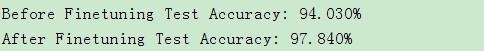
但是微调后的结果基本是一样的。
PS:讲义地址:http://deeplearning.stanford.edu/wiki/index.php/Exercise:_Implement_deep_networks_for_digit_classification
