Creating publication-quality output
The Sweave package allows you to embed R code and output in LaTeX documents, in order to produce high-end typeset reports in PDF, PostScript, and DVI formats. Sweave is an elegant, precise, and highly flexible system,but it requires the author to be conversant with LaTeX coding
In a similar fashion, the odfWeave package provides a mechanism for embedding R code and output in documents that follow the Open Documents Format ( ODF).These reports can be further edited via an ODF word processor, such as OpenOffice Writer, and saved in either ODF or Microsoft Word format. The process is not as flexible as the Sweave approach, but it eliminates the need to learn LaTeX.
High-quality typesetting with Sweave (R + LaTeX)
LaTeX is a document preparation system for high-quality typesetting
(http://www.latex-project.org)
The Sweave package allows you to embed R code and output (including graphs) within the LaTeX document. This is a multistep process:
1 A special document called a noweb file (typically with the extension .Rnw) is created using any text editor. The file contains the written content, LaTeX markup code , and R code chunks. Each R code chunk starts with the delimiter <<>>= and ends with the delimiter @.
2 The Sweave() function processes the noweb file and generates a LaTeX file. During this step, the R code chunks are processed, and depending on options, replaced with LaTeX-formatted R code and output. This step can be accomplished from within R or from the command line.
Sweave("infile.Rnw")
By default, Sweave("example.Rnw") would input the file example.Rnw from the current working directory and output the file example.tex to the same directory.
Alternatively, use can use
Sweave("infile.Rnw", syntax="SweaveSyntaxNoweb")
Specifying this syntax option can help avoid some common parsing errors, as well
as conflicts with the R2HTML package .
Execution from the command line will depend on the operating system. For example, on a Linux system, this might look like $ R CMD Sweave infile.Rnw
3 The LaTeX file is then run through a LaTeX compiler, creating a PDF, PostScript, or DVI file. Popular LaTeX compilers include TeX Live for Linux, MacTeX for Mac, and proTeXt for Windows.
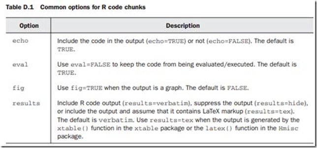
As indicated earlier, each chunk of R code is surrounded by <<>>= and @. You can add options to each <<>>= delimiter in order to control the processing of the corresponding R code chunk. For example
<<echo=TRUE, results=HIDE>>=
summary(lm(Y~X, data=mydata))
@
would output the code, but not the results, whereas
<<echo=FALSE, fig=TRUE>>=
plot(A)
@
wouldn’t print the code but would include the graph in the output.
By default, Sweave will add LaTeX markup code to attractively format data frames, matrices, and vectors.
Additionally, R objects can be embedded inline using a \Sexpr{} statement .
Note that lattice graphs must be embedded in a print() statement to be processed properly.
The xtable() function in the xtable package can be used to format data frames and matrices more precisely. In addition, it can be used to format other R objects, including those produced by lm(), glm(), aov(), table(), ts(), and coxph().
Use method(xtable) to view a comprehensive list. When formatting R output using
xtable() , be sure to include the results=tex option in the code chunk delimiter.
A sample noweb file (example.nrw)
\documentclass[12pt]{article}
\title{Sample Report}
\author{Robert I. Kabacoff, Ph.D.}
\date{}
\begin{document}
\maketitle
<<echo=false, results=hide>>=
library(multcomp)
library(xtable)
attach(cholesterol)
@
\section{Results}
Cholesterol reduction was assessed in a study
that randomized \Sexpr{nrow(cholesterol)} patients
to one of \Sexpr{length(unique(trt))} treatments.
Summary statistics are provided in
Table \ref{table:descriptives}.
<<echo = false, results = tex>>=
descTable <- data.frame("Treatment" = sort(unique(trt)),
"N" = as.vector(table(trt)),
"Mean" = tapply(response, list(trt), mean, na.rm=TRUE),
"SD" = tapply(response, list(trt), sd, na.rm=TRUE)
)
print(xtable(descTable, caption = "Descriptive statistics
for each treatment group", label = "table:descriptives"),
caption.placement = "top", include.rownames = FALSE)
@
The analysis of variance is provided in Table \ref{table:anova}.
<<echo=false, results=tex>>=
fit <- aov(response ~ trt)
print(xtable(fit, caption = "Analysis of variance",
label = "table:anova"), caption.placement = "top")
@
\noindent and group differences are plotted in Figure \ref{figure:tukey}.
\begin{figure}\label{figure:tukey}
\begin{center}
<<fig=TRUE,echo=FALSE>>=
par(mar=c(5,4,6,2))
tuk <- glht(fit, linfct=mcp(trt="Tukey"))
plot(cld(tuk, level=.05),col="lightgrey",xlab="Treatment", ylab="Response")
box("figure")
@
\caption{Distribution of response times and pairwise comparisons.}
\end{center}
\end{figure}
\end{document}
www.stat.uni-muenchen.de/~leisch/Sweave
http://biostat.mc.vanderbilt.edu/TheresaScott
"The Not So Short Introduction to LaTeX 2e,” www.latex-project.org
The packages R2wd and R2PPT can be used to dynamically create Word and PowerPoint documents with inserted R output, but they are in their formative stages of development.


