机器学习算法原理实现——线性判别分析LDA

介绍

线性判别分析（Linear Discriminant Analysis, LDA）是一种有监督式的数据降维方法，是在机器学习和数据挖掘中一种广泛使用的经典算法。
LDA的希望将带上标签的数据（点），通过投影的方法，投影到维度更低的空间中，使得投影后的点，按类别区分成一簇一簇的情况，并且相同类别的点，将会在投影后的空间中更接近。

 

如上图所示（数据只有二维的情况），LDA希望能寻找到第二条直线，并将高维的数据投影到低维空间中，使得类之间耦合度低，类内的聚合度高。这样的话，接下来就可以方便利用低维的数据对数据进行分类。

理论基础

见: https://leondong1993.github.io/2017/05/lda/ 讲解比较清楚！

核心就是求解一个n*k矩阵将原来n维的数据降到k维，也就是说把原始数据降低到了k维。

 

一个简单的例子

假设我现在有两类数据，如下图所示。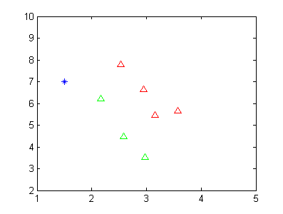

其中红色的三角形代表一类数据，绿色的三角形代表第二类数据。蓝色的点代表未知样本点，我想通过LDA的方式判断其类别。当然从这个二维图中，我们可以看到该蓝色的数据点应该是属于第二类的（绿色）。

LDA得到两类数据的一维表示，如下图所示。

 

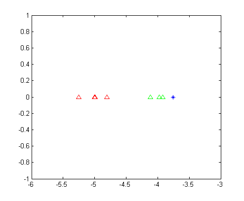
从这幅图里面我们可以清晰的看出，第一类数据和第二类数据被完美的分开了，并且可以明显的看出来，位置数据应该是属于第二类的。

 

代码参考：

?

1 2 3 4 5 6 7 8 9 10 11 12 13 14 15 16 17 18 19 20 21 22 23 24 25 26 27 28 29 30 31 32 33 34 35 36 37 38 39 40 41 42 43 44 45 46 47 48 49 50 51 52 53 54 55 56 57 58 59 60 61 62 63 64 65 66 67 68 69 70 71 72 73 74 75 76 77 78 79 80 81 82 83 84 85 86 87 88 89 90 91 92 93 94

import numpy as np   ### 定义LDA类 class LDA:     def __init__(self):         # 初始化权重矩阵         self.w = None           # 协方差矩阵计算方法     def calc_cov(self, X, Y=None):         m = X.shape[0]         # 数据标准化         X = (X - np.mean(X, axis=0))/np.std(X, axis=0)         Y = X if Y == None else \             (Y - np.mean(Y, axis=0))/np.std(Y, axis=0)         return 1 / m * np.matmul(X.T, Y)           # 数据投影方法     def project(self, X, y):         # LDA拟合获取模型权重         self.fit(X, y)         # 数据投影         X_projection = X.dot(self.w)         return X_projection           # LDA拟合方法     def fit(self, X, y):         # (1) 按类分组         X0 = X[y == 0]         X1 = X[y == 1]         # (2) 分别计算两类数据自变量的协方差矩阵         sigma0 = self.calc_cov(X0)         sigma1 = self.calc_cov(X1)         # (3) 计算类内散度矩阵         Sw = sigma0 + sigma1         # (4) 分别计算两类数据自变量的均值和差         u0, u1 = np.mean(X0, axis=0), np.mean(X1, axis=0)         mean_diff = np.atleast_1d(u0 - u1)         # (5) 对类内散度矩阵进行奇异值分解         U, S, V = np.linalg.svd(Sw)         # (6) 计算类内散度矩阵的逆         Sw_ = np.dot(np.dot(V.T, np.linalg.pinv(np.diag(S))), U.T)         # (7) 计算w         self.w = Sw_.dot(mean_diff)           # LDA分类预测     def predict(self, X):         # 初始化预测结果为空列表         y_pred = []         # 遍历待预测样本         for x_i in X:             # 模型预测             h = x_i.dot(self.w)             y = 1 * (h < 0)             y_pred.append(y)         return y_pred         # 导入LinearDiscriminantAnalysis模块 from sklearn.discriminant_analysis import LinearDiscriminantAnalysis   # 导入相关库 from sklearn import datasets from sklearn.model_selection import train_test_split from sklearn.metrics import accuracy_score # 导入iris数据集 data = datasets.load_iris() # 数据与标签 X, y = data.data, data.target # 取标签不为2的数据 X = X[y != 2] y = y[y != 2] # 划分训练集和测试集 X_train, X_test, y_train, y_test = train_test_split(X, y, test_size=0.2, random_state=41) # 创建LDA模型实例 lda = LDA() # LDA模型拟合 lda.fit(X_train, y_train) # LDA模型预测 y_pred = lda.predict(X_test) # 测试集上的分类准确率 acc = accuracy_score(y_test, y_pred) print("Accuracy of NumPy LDA:", acc)     # 创建LDA分类器 clf = LinearDiscriminantAnalysis() # 模型拟合 clf.fit(X_train, y_train) # 模型预测 y_pred = clf.predict(X_test) # 测试集上的分类准确率 acc = accuracy_score(y_test, y_pred) print("Accuracy of Sklearn LDA:", acc)

　　

好难！还有一些实现：

https://python-course.eu/machine-learning/linear-discriminant-analysis-in-python.php

https://www.adeveloperdiary.com/data-science/machine-learning/linear-discriminant-analysis-from-theory-to-code/

?

1 2 3 4 5 6 7 8 9 10 11 12 13 14 15 16 17 18 19 20 21 22 23 24 25 26 27 28 29 30 31 32 33 34 35 36 37 38 39 40 41 42 43 44 45 46 47 48 49 50 51 52 53 54 55 56 57 58 59 60 61 62 63 64 65 66 67 68 69 70 71 72 73 74 75 76 77 78 79 80 81 82 83 84 85 86 87 88 89 90 91 92 93 94 95 96 97 98 99 100 101 102 103 104 105 106 107 108 109 110 111 112 113 114 115 116 117 118 119 120 121 122 123 124 125 126 127 128 129 130 131 132 133 134 135 136 137

import numpy as np import matplotlib.pyplot as plt from sklearn import preprocessing import seaborn as sns     def load_data(cols, load_all=False, head=False):     iris = sns.load_dataset("iris")       if not load_all:         if head:             iris = iris.head(100)         else:             iris = iris.tail(100)       le = preprocessing.LabelEncoder()     y = le.fit_transform(iris["species"])       X = iris.drop(["species"], axis=1)       if len(cols) > 0:         X = X[cols]       return X.values, y     class LDA:     def __init__(self):         pass       def fit(self, X, y):         target_classes = np.unique(y)           mean_vectors = []           for cls in target_classes:             mean_vectors.append(np.mean(X[y == cls], axis=0))           if len(target_classes) < 3:             mu1_mu2 = (mean_vectors[0] - mean_vectors[1]).reshape(1, X.shape[1])             B = np.dot(mu1_mu2.T, mu1_mu2)         else:             data_mean = np.mean(X, axis=0).reshape(1, X.shape[1])             B = np.zeros((X.shape[1], X.shape[1]))             for i, mean_vec in enumerate(mean_vectors):                 n = X[y == i].shape[0]                 mean_vec = mean_vec.reshape(1, X.shape[1])                 mu1_mu2 = mean_vec - data_mean                   B += n * np.dot(mu1_mu2.T, mu1_mu2)           s_matrix = []           for cls, mean in enumerate(mean_vectors):             Si = np.zeros((X.shape[1], X.shape[1]))             for row in X[y == cls]:                 t = (row - mean).reshape(1, X.shape[1])                 Si += np.dot(t.T, t)             s_matrix.append(Si)           S = np.zeros((X.shape[1], X.shape[1]))         for s_i in s_matrix:             S += s_i           S_inv = np.linalg.inv(S)           S_inv_B = S_inv.dot(B)           eig_vals, eig_vecs = np.linalg.eig(S_inv_B)           idx = eig_vals.argsort()[::-1]           eig_vals = eig_vals[idx]         eig_vecs = eig_vecs[:, idx]           return eig_vecs     # Experiment 1 # cols = ["petal_length", "petal_width"] # X, y = load_data(cols, load_all=False, head=True) # print(X.shape)   # lda = LDA() # eig_vecs = lda.fit(X, y) # W = eig_vecs[:, :1]   # colors = ['red', 'green', 'blue'] # fig, ax = plt.subplots(figsize=(10, 8)) # for point, pred in zip(X, y): #     ax.scatter(point[0], point[1], color=colors[pred], alpha=0.3) #     proj = (np.dot(point, W) * W) / np.dot(W.T, W)   #     ax.scatter(proj[0], proj[1], color=colors[pred], alpha=0.3)   # plt.show()   # Experiment 2 # cols = ["petal_length", "petal_width"] # X, y = load_data(cols, load_all=True, head=True) # print(X.shape)   # lda = LDA() # eig_vecs = lda.fit(X, y) # W = eig_vecs[:, :1]   # colors = ['red', 'green', 'blue'] # fig, ax = plt.subplots(figsize=(10, 8)) # for point, pred in zip(X, y): #     ax.scatter(point[0], point[1], color=colors[pred], alpha=0.3) #     proj = (np.dot(point, W) * W) / np.dot(W.T, W)   #     ax.scatter(proj[0], proj[1], color=colors[pred], alpha=0.3)   # plt.show()   # Experiment 3 X, y = load_data([], load_all=True, head=True) print(X.shape)   lda = LDA() eig_vecs = lda.fit(X, y) W = eig_vecs[:, :2]   transformed = X.dot(W)   plt.scatter(transformed[:, 0], transformed[:, 1], c=y, cmap=plt.cm.Set1) plt.show()   from sklearn.discriminant_analysis import LinearDiscriminantAnalysis   clf = LinearDiscriminantAnalysis() clf.fit(X, y) transformed = clf.transform(X)   plt.scatter(transformed[:, 0], transformed[:, 1], c=y, cmap=plt.cm.Set1) plt.show()