
ART使用课程——IBM的ART工具很强啊,真正能够用于安全AI模型对抗的实用工具
Adversarial Robustness Toolbox 是 IBM 研究团队开源的用于检测模型及对抗攻击的工具箱,为开发人员加强 AI
模型被误导的防御性,让 AI 系统变得更加安全,目前支持 TensorFlow 和 Keras 框架,未来预计会支持更多框架。
支持以下攻击和防御的方法
-
Deep Fool
-
Fast Gradient Method
-
Jacobian Saliency Map
-
Universal Perturbation
-
Virtual Adversarial Method
-
C&W Attack
-
NewtonFool
防御方法
-
Feature squeezing
-
Spatial smoothing
-
Label smoothing
-
Adversarial training
-
Virtual adversarial training
https://github.com/Trusted-AI/adversarial-robustness-toolbox
ART for Red and Blue Teams (selection)

Learn more
| Get Started | Documentation | Contributing |
|---|---|---|
| - Installation - Examples - Notebooks |
- Attacks - Defences - Estimators - Metrics - Technical Documentation |
- Slack, Invitation - Contributing - Roadmap - Citing |
第三种:对抗训练-规避攻击的对策-
您可以使用 ART 来验证针对 AI 的攻击方法(恶意样本攻击、数据污染攻击、模型提取、成员推断等)以及针对它们的防御方法。为了保护人工智能免受攻击,有必要了解攻击的机制和适当的防御方法。因此,在本专栏中,我们将学习通过 ART来确保 AI 安全的技术。
在第三节课中,我们将练习对抗性训练,这是针对规避攻击的对策之一。
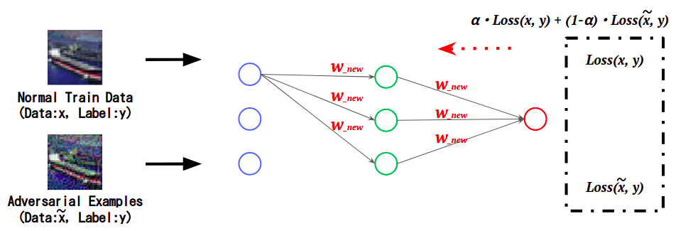
对抗训练是一种增强人工智能鲁棒性的防御方法,通过在学习过程中学习敌对样本的特征,抑制敌对样本的错误分类。
下图通过计算正常数据和敌对样本在学习AI时的误差(Loss),并根据附加值更新AI权重,展示了敌对样本的特征。
- 对抗训练的概念图

这样,已经学习到敌对样本特征的AI将敌对样本分类到正确的(原始)类中。这一次,我们将使用
在 ART 中实施的Ensemble Adversarial Training来练习 Adversarial Training。
| * 1 .. 本栏目中AI的定义 |
|---|
| 在本专栏中,可以执行通常需要人类智能的任务的计算机系统,例如图像分类和语音识别,特别是使用机器学习创建的系统,将被称为“AI”。 |
| 笔记 |
|---|
| 本专栏旨在帮助您了解确保 AI 安全的技术。核实本栏目内容时,请务必使用您控制的系统,并自行承担风险。如果您未经许可在第三方系统上运行它,您可能会受到法律的惩罚。 |
为了更深入地了解本专栏的内容,最好对敌对样本有一个基本的了解。
如果您不知道敌对样本,请提前查看AI安全超级介绍:第2部分AI欺骗攻击-敌对样本- 。
动手
本专栏将以实践形式进行,因为它强调通过实践学习 ART。
可以在您自己的环境或作者准备的Google Colaboratory * 2中执行动手操作。
如果您想使用 Google Colaboratory 进行动手操作,请访问以下 URL。
Google Colaboratory: ART Super Introduction-Part 3: Countermeasures for Avoidance Attacks Adversarial Training-
| * 2: 使用 Colaboratory |
|---|
| 您需要一个 Google 帐户才能使用 Google Colaboratory。 如果您没有,请先创建一个 Google 帐户。 |
如果您想在自己的环境中动手操作,请按照以下说明执行代码。
提前准备
安装 ART
ART 不是 Python 的内置库,因此请安装它。
# [1-1]
# ARTのインストール。
pip3 install adversarial-robustness-toolbox
库导入
导入构建 ART 和图像分类器所需的库。
在本次实践中,我们将导入 Keras 类,以使用 TensorFlow 中内置的 Keras 构建图像分类器。
此外,导入在 ART中执行对抗训练AdversarialTrainer的类。
# [1-2]
# 必要なライブラリのインポート
import random
import numpy as np
import matplotlib.pyplot as plt

# TensorFlow with Keras.
import tensorflow as tf
from tensorflow.keras.models import Model
from tensorflow.keras.layers import Input, Dense, Conv2D
from tensorflow.keras.layers import MaxPooling2D, GlobalAveragePooling2D, Dropout
tf.compat.v1.disable_eager_execution()

# ART
from art.defences.trainer import AdversarialTrainer
from art.attacks.evasion import FastGradientMethod
from art.estimators.classification import KerasClassifier
数据集加载
使用 CIFAR10 作为目标图像分类器的训练数据。
# [1-3]
# CIFAR10のロード。
(X_train, y_train), (X_test, y_test) = tf.keras.datasets.cifar10.load_data()

# CIFAR10のラベル。
classes = ['airplane', 'automobile', 'bird', 'cat', 'deer', 'dog', 'frog', 'horse', 'ship', 'truck']
num_classes = len(classes)
检查 CIFAR10 的记录图像。
从加载的数据集中随机抽取 25 张图像并显示在屏幕上。
# [1-4]
# データセットの可視化。
show_images = []
for _ in range(5 * 5):
    show_images.append(X_train[random.randint(0, len(X_train))])

for idx, image in enumerate(show_images):
    plt.subplot(5, 5, idx + 1)
    plt.imshow(image)

# 学習データ数、テストデータ数を表示。
print(X_train.shape, y_train.shape)
CIFAR10'airplane', 'automobile', 'bird', 'cat', 'deer', 'dog', 'frog', 'horse', 'ship', 'truck'包含 10 个类别的 60,000 张图像。
细分为学习数据:50,000 张,测试数据:10,000 张,每张图像为 32 x 32 像素的 RGB 格式。
数据集预处理
规范化数据集并将标签转换为One-hot-vector格式。
# [1-5]
# 正規化。
X_train = X_train.astype('float32') / 255
X_test = X_test.astype('float32') / 255

# ラベルをOne-hot-vector化。
y_train = tf.keras.utils.to_categorical(y_train, num_classes)
y_test = tf.keras.utils.to_categorical(y_test, num_classes)
创建攻击目标模型
创建图像分类器以针对规避攻击。
模型定义
在本次动手实践中,定义了以下 CNN(卷积神经网络)。
# [1-6]
# モデルの定義。
def define_model():
    inputs = Input(shape=(32, 32, 3))
    x = Conv2D(64, (3, 3), padding='SAME', activation='relu')(inputs)
    x = Conv2D(64, (3, 3), padding='SAME', activation='relu')(x)
    x = Dropout(0.25)(x)
    x = MaxPooling2D()(x)

    x = Conv2D(128, (3,3), padding='SAME', activation='relu')(x)
    x = Conv2D(128, (3,3), padding='SAME', activation='relu')(x)
    x = Dropout(0.25)(x)
    x = MaxPooling2D()(x)

    x = Conv2D(256, (3,3), padding='SAME', activation='relu')(x)
    x = Conv2D(256, (3,3), padding='SAME', activation='relu')(x)
    x = GlobalAveragePooling2D()(x)

    x = Dense(1024, activation='relu')(x)
    x = Dropout(0.25)(x)
    y = Dense(10, activation='softmax')(x)

    model = Model(inputs, y)

    # モデルのコンパイル。
    model.compile(optimizer=tf.keras.optimizers.Adam(),
                  loss='categorical_crossentropy',
                  metrics=['accuracy'])
    model.summary()
    return model

model = define_model()
应用 Keras 分类器
为了在 ART 中进行对抗训练,有必要将受保护的图像分类器包装在 ART 提供的包装类中。
https://adversarial-robustness-toolbox.readthedocs.io/en/latest/modules/estimators/classification.html#keras-classifier
ART 有一个类,封装了由 TensorFlow、PyTorch、Scikit-learn 等各种框架创建的模型,但在本次动手中,由于分类器是使用 Keras 创建的,因此KerasClassifier使用 . 来做。
- KerasClassifier 参数
model:指定要攻击的训练分类器。clip_values:指定输入数据特征的最小值和最大值。use_logits: 如果分类器的输出格式是 Logit,则指定 True,如果输出格式是概率值,则指定 False。
# [1-7]
# 入力データの特徴量の最小値・最大値を指定。
# 特徴量は0.0~1.0の範囲に収まるように正規化しているため、最小値は0.0、最大値は1.0とする。
min_pixel_value = 0.0
max_pixel_value = 1.0

# モデルをART Keras Classifierでラップ。
classifier = KerasClassifier(model=model, clip_values=(min_pixel_value, max_pixel_value), use_logits=False)
模型学习
训练数据X_train, y_train用于训练图像分类器。
epoch 的数量设置为 30 以减少动手时间。
# [1-8]
# 学習の実行。
classifier.fit(X_train, y_train,
               batch_size=512,
               nb_epochs=30,
               validation_data=(X_test, y_test),
               shuffle=True)
模型精度评估
使用测试数据X_test评估创建的图像分类器的推理精度。
# [1-9]
# モデルの精度評価。
predictions = classifier.predict(X_test)
accuracy = np.sum(np.argmax(predictions, axis=1) == np.argmax(y_test, axis=1)) / len(y_test)
print('Accuracy on benign test example: {}%'.format(accuracy * 100))
推理准确率大概在80% 左右。
创建敌对样本
使用 ART创建规避攻击的敌对样本。
运行 FGSM
使用 ART 中实现的 FGSM 创建一个敌对样本。
https://adversarial-robustness-toolbox.readthedocs.io/en/latest/modules/attacks/evasion.html#fast-gradient-method-fgm
FastGradientMethod将包装分类器和扰动量(小的变化)指定为FGSM 类的参数。
FastGradientMethod参数estimator:指定攻击目标分类器被包装KerasClassifier。eps:指定要添加到敌对样本的扰动量。
# [1-10]
# FGSMインスタンスの作成。
attack = FastGradientMethod(estimator=classifier, eps=0.1)
如上所述,FastGradientMethod您可以简单地通过为参数指定所需的参数来创建恶意样本。攻击的成功率(导致错误分类的概率)
与第二个参数中指定的值成比例增加,但图像看起来不自然(因为噪声增加)。因此,攻击的成功率与敌对样本的自然外观之间存在权衡。eps
然后使用 FGSM 实例的方法generate生成恶意样本。
generate参数x:指定作为敌对样本基础的正常数据(图像)。
# [1-11]
# 敵対的サンプルの生成(ベース画像はテストデータとする)。
X_test_adv = attack.generate(x=X_test)
执行推理
将生成的敌对样本输入图像分类器并评估推理精度。
# [1-12]
# 敵対的サンプルを使用して画像分類器の推論精度を評価。
all_preds = classifier.predict(X_test_adv)
accuracy = np.sum(np.argmax(all_preds, axis=1) == np.argmax(y_test, axis=1)) / len(y_test)
print('Accuracy on Adversarial Exmaples: {}%'.format(accuracy * 100))
可以看到,与正常测试数据的情况相比,推理准确度显着降低。
从这个结果可以推断出恶意样本会导致错误分类。
接下来,目视检查正常数据和敌对样本的推理结果。
首先,推断正常数据。
# [1-13]
# 正常なデータ(摂動が加えられる前のデータ)。
target_index = 2
plt.imshow(X_test[target_index])

# 正常データの推論
pred = classifier.predict(X_test[target_index][np.newaxis, ...])

# 推論結果の表示。
print('True label: "{}"\nPrediction: "{}"'.format(classes[np.argmax(y_test[target_index])], classes[np.argmax(pred)]))
显示的图像是输入到图像分类器的正常数据。
也许True label图像分类器的实际标签和预测标签Prediction匹配。
然后推断出敌对样本。
# [1-14]
# 敵対的サンプル。
plt.imshow(X_test_adv[target_index])

# 敵対的サンプルの推論。
pred_adv = classifier.predict(X_test_adv[target_index][np.newaxis, ...])

# 推論結果の表示。
print('True label: "{}"\nPrediction: "{}"'.format(classes[np.argmax(y_test[target_index])], classes[np.argmax(pred_adv)]))
显示的图像是图像分类器的恶意样本输入。
由于扰动的影响,存在噪音,但True label我认为它看起来像中所示的图像。
但是,我不认为图像分类器的实际标签True label和预测标签匹配。这样,通过使用 FGSM 添加扰动,我们可以看到它们被错误分类为与人类外观不同的类别。* 如果攻击不顺利,请尝试通过反复试验更改 [1-13]或 [1-10] 。Predictiontarget_indexeps
对抗训练
使用 ART 进行对抗训练。
应用对抗训练师
ART 有一个对抗训练类AdversarialTrainer,所以我们将使用它。
https://adversarial-robustness-toolbox.readthedocs.io/en/latest/modules/defences/trainer.html#adversarial-training
AdversarialTrainer的论点- 分类器:指定要保护的模型。
在本次实践中,我们将创建一个新的分类器robustness_classifier并应用对抗训练。 - 攻击:指定创建恶意样本的实例。
在本实践中,指定在 [1-10] 中创建FastGradientMethod的实例。 - ratio:指定用于创建恶意样本的数据与训练数据的比率。
例如)ratio=0.5,一半的训练数据将用于敌对样本的创建和对抗训练。
- 分类器:指定要保护的模型。
# [1-15]
# Adversarial Trainingインスタンスの作成。
robustness_classifier = KerasClassifier(model=define_model(), clip_values=(min_pixel_value, max_pixel_value), use_logits=False)
defense = AdversarialTrainer(classifier=robustness_classifier, attacks=attack, ratio=0.5)
进行对抗训练
使用训练数据X_train, y_train对图像分类器执行对抗训练。
请注意,对抗训练可能需要一个小时或更长时间。
如果您在运行时遇到 Google Colab 会话中断,请尝试减少 epoch 数以减少执行时间(尽管这会降低您对恶意样本的抵抗力)。
# [1-16]
# Adversarial Trainingの実行。
defense.fit(X_train, y_train,
            batch_size=512,
            nb_epochs=30,
            validation_data=(X_test, y_test),
            shuffle=True)
模型精度评估
使用测试数据X_test和敌对样本X_test_adv评估图像分类器的准确性。为了比较,我们还评估了
没有对抗训练的图像分类器的准确性。classifier
# [1-17]
# Adversarial Trainingを適用していない分類器「classifier」。
# テストデータの推論精度を評価。
all_preds = classifier.predict(X_test)
accuracy = np.sum(np.argmax(all_preds, axis=1) == np.argmax(y_test, axis=1)) / len(y_test)
print('Vulnerable classifier: Accuracy on test example: {}%'.format(accuracy * 100))

# 敵対的サンプルの推論精度を評価。
all_preds = classifier.predict(X_test_adv)
accuracy = np.sum(np.argmax(all_preds, axis=1) == np.argmax(y_test, axis=1)) / len(y_test)
print('Vulnerable classifier: Accuracy on Adversarial Exmaples: {}%'.format(accuracy * 100))

# Adversarial Trainingを適用した分類器「defense」。
# テストデータの推論精度を評価。
all_preds = defense.predict(X_test)
accuracy = np.sum(np.argmax(all_preds, axis=1) == np.argmax(y_test, axis=1)) / len(y_test)
print('Robustness classifier: Accuracy on test example: {}%'.format(accuracy * 100))

# 敵対的サンプルの推論精度を評価。
all_preds = defense.predict(X_test_adv)
accuracy = np.sum(np.argmax(all_preds, axis=1) == np.argmax(y_test, axis=1)) / len(y_test)
print('Robustness classifier: Accuracy on Adversarial Exmaples: {}%'.format(accuracy * 100))
Vulnerable classifier~表示的部分是图像分类器在没有应用 Adversarial Training 的情况下的推理精度。
可以看出,正常数据的推理准确率在80%左右,敌对样本的推理准确率明显偏低(大概在10%左右)。
另一方面,Robustness classifier~由 表示的部分是应用对抗训练的图像分类器的推理精度。
可以看出,正常数据的推理准确率在80%左右,敌对样本的推理准确率在70-80%左右(*)。推理准确率Vulnerable classifier~比. * 在本次动手实践中,减少了 epoch 的数量以缩短时间,但可以通过增加 Adversarial Training 中的 epoch 数量和调整 [1-15] 来进一步提高推理精度。ratio
此外,虽然这次没有实践,但 ART 还提供了一种在增强训练数据的同时执行对抗训练的方法。
通过使用这种方法,似乎可以进一步提高推理精度。
https://adversarial-robustness-toolbox.readthedocs.io/en/latest/modules/defences/trainer.html#art.defences.trainer.AdversarialTrainer.fit_generator
综上所述
在本次实践中,我们以“3rd-Countermeasures against evasive attack Adversarial Training-”为题,练习了一种防御方法,通过将训练数据与敌对样本混合来增加对规避攻击的抵抗力。
结果发现,可以显着提高敌对样本的推理精度。
这样就可以很方便的使用ART进行AI安全测试,有兴趣的小伙伴推荐试试。
就这样

 浙公网安备 33010602011771号