图卷积神经网络——咋感觉就是做词嵌入 然后给出分类结果呢 类似deepwalk+分类

推荐系统

在电子商务平台中，用户与产品的交互构成图结构，因此许多公司使用图神经网络进行产品推荐。典型的做法是对用户和商品的交互关系进行建模，然后通过某种负采样损失学习节点嵌入，并通过kNN实时推荐给用户相似产品。Uber Eats公司很早就通过这样的方式进行产品推荐，具体而言，他们使用图神经网络 GraphSage 为用户推荐食品和餐厅。

在食品推荐中，由于地理位置的限制，使用的图结构比较小。在一些包含数10亿节点的大规模图上，同样也可以使用图神经网络。使用传统方法处理如此大规模的图是非常困难的，阿里巴巴公司在包含数十亿用户和产品的网络上研究图嵌入和GNN，最近他们提出的Aligraph，仅需要五分钟就可以构建具有400M节点的图。非常强大！此外，Aligraph还支持高效的分布式图存储，对采样过程进行了优化，同时内部集成了很多GNN模型。该框架已成功用于公司的多种产品推荐和个性化搜索任务。

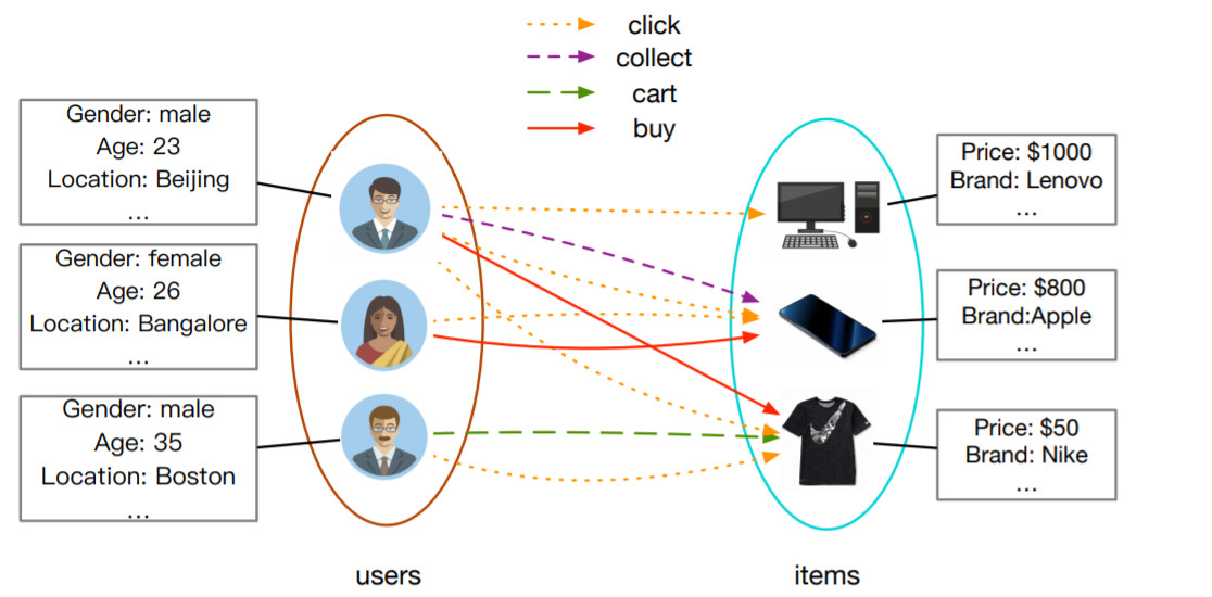
Alibaba,Amazon以及其他很多电子商务平台使用GNN构建推荐系统

Pinterest 提出了 PinSage 模型，该模型使用个性化PageRank对邻域进行高效采样，并通过聚合邻域更新节点嵌入。后续模型 PinnerSage 进一步扩展了该框架来处理不同用户的多嵌入问题。受限篇幅，本文仅列出GNN在推荐系统的部分应用，但这些足以表明，如果用户互动的信息足够丰富，那么GNNs将显著推动推荐系统中进一步发展。

GRAPH CONVOLUTIONAL NETWORKS

THOMAS KIPF, 30 SEPTEMBER 2016

Multi-layer Graph Convolutional Network (GCN) with first-order filters.

Overview

Many important real-world datasets come in the form of graphs or networks: social networks, knowledge graphs, protein-interaction networks, the World Wide Web, etc. (just to name a few). Yet, until recently, very little attention has been devoted to the generalization of neural network models to such structured datasets.

In the last couple of years, a number of papers re-visited this problem of generalizing neural networks to work on arbitrarily structured graphs (Bruna et al., ICLR 2014; Henaff et al., 2015; Duvenaud et al., NIPS 2015; Li et al., ICLR 2016; Defferrard et al., NIPS 2016; Kipf & Welling, ICLR 2017), some of them now achieving very promising results in domains that have previously been dominated by, e.g., kernel-based methods, graph-based regularization techniques and others.

In this post, I will give a brief overview of recent developments in this field and point out strengths and drawbacks of various approaches. The discussion here will mainly focus on two recent papers:

• Kipf & Welling (ICLR 2017), Semi-Supervised Classification with Graph Convolutional Networks (disclaimer: I'm the first author)
• Defferrard et al. (NIPS 2016), Convolutional Neural Networks on Graphs with Fast Localized Spectral Filtering

and a review/discussion post by Ferenc Huszar: How powerful are Graph Convolutions? that discusses some limitations of these kinds of models. I wrote a short comment on Ferenc's review here (at the very end of this post).

Outline

• Short introduction to neural network models on graphs
• Spectral graph convolutions and Graph Convolutional Networks (GCNs)
• Demo: Graph embeddings with a simple 1st-order GCN model
• GCNs as differentiable generalization of the Weisfeiler-Lehman algorithm

If you're already familiar with GCNs and related methods, you might want to jump directly to Embedding the karate club network.

How powerful are Graph Convolutional Networks?

Recent literature

Generalizing well-established neural models like RNNs or CNNs to work on arbitrarily structured graphs is a challenging problem. Some recent papers introduce problem-specific specialized architectures (e.g. Duvenaud et al., NIPS 2015; Li et al., ICLR 2016; Jain et al., CVPR 2016), others make use of graph convolutions known from spectral graph theory1 (Bruna et al., ICLR 2014; Henaff et al., 2015) to define parameterized filters that are used in a multi-layer neural network model, akin to "classical" CNNs that we know and love.

More recent work focuses on bridging the gap between fast heuristics and the slow2, but somewhat more principled, spectral approach. Defferrard et al. (NIPS 2016) approximate smooth filters in the spectral domain using Chebyshev polynomials with free parameters that are learned in a neural network-like model. They achieve convincing results on regular domains (like MNIST), closely approaching those of a simple 2D CNN model.

In Kipf & Welling (ICLR 2017), we take a somewhat similar approach and start from the framework of spectral graph convolutions, yet introduce simplifications (we will get to those later in the post) that in many cases allow both for significantly faster training times and higher predictive accuracy, reaching state-of-the-art classification results on a number of benchmark graph datasets.

GCNs Part I: Definitions

Currently, most graph neural network models have a somewhat universal architecture in common. I will refer to these models as Graph Convolutional Networks (GCNs); convolutional, because filter parameters are typically shared over all locations in the graph (or a subset thereof as in Duvenaud et al., NIPS 2015).

For these models, the goal is then to learn a function of signals/features on a graph G=(V,E)G=(V,E) which takes as input:

• A feature description xixi for every node ii; summarized in a N×DN×D feature matrix XX (NN: number of nodes, DD: number of input features)
• A representative description of the graph structure in matrix form; typically in the form of an adjacency matrix AA (or some function thereof)

and produces a node-level output ZZ (an N×FN×F feature matrix, where FF is the number of output features per node). Graph-level outputs can be modeled by introducing some form of pooling operation (see, e.g. Duvenaud et al., NIPS 2015).

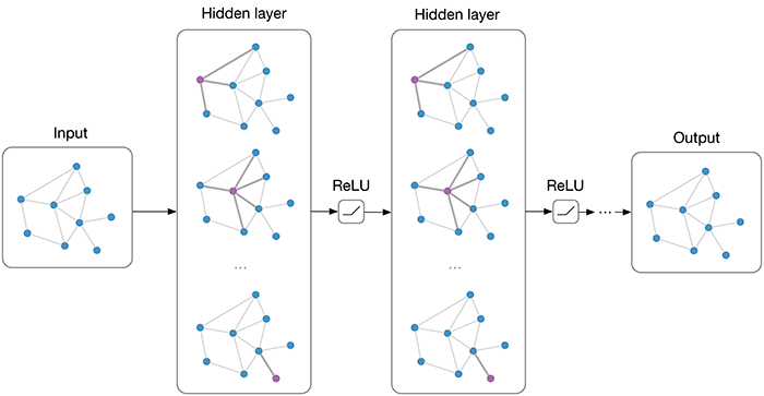
Every neural network layer can then be written as a non-linear function

H(l+1)=f(H(l),A),H(l+1)=f(H(l),A),

with H(0)=XH(0)=X and H(L)=ZH(L)=Z (or zz for graph-level outputs), LL being the number of layers. The specific models then differ only in how f(⋅,⋅)f(⋅,⋅) is chosen and parameterized.

 

GCNs Part II: A simple example

As an example, let's consider the following very simple form of a layer-wise propagation rule:

 

f(H(l),A)=σ(AH(l)W(l)),f(H(l),A)=σ(AH(l)W(l)),

 

where W(l)W(l) is a weight matrix for the ll-th neural network layer and σ(⋅)σ(⋅) is a non-linear activation function like the ReLUReLU. Despite its simplicity this model is already quite powerful (we'll come to that in a moment).

But first, let us address two limitations of this simple model: multiplication with AA means that, for every node, we sum up all the feature vectors of all neighboring nodes but not the node itself (unless there are self-loops in the graph). We can "fix" this by enforcing self-loops in the graph: we simply add the identity matrix to AA.

The second major limitation is that AA is typically not normalized and therefore the multiplication with AA will completely change the scale of the feature vectors (we can understand that by looking at the eigenvalues of AA). Normalizing AA such that all rows sum to one, i.e. D−1AD−1A, where DD is the diagonal node degree matrix, gets rid of this problem. Multiplying with D−1AD−1A now corresponds to taking the average of neighboring node features. In practice, dynamics get more interesting when we use a symmetric normalization, i.e. D−12AD−12D−12AD−12 (as this no longer amounts to mere averaging of neighboring nodes). Combining these two tricks, we essentially arrive at the propagation rule introduced in Kipf & Welling (ICLR 2017):

 

f(H(l),A)=σ(D^−12A^D^−12H(l)W(l)),f(H(l),A)=σ(D^−12A^D^−12H(l)W(l)),

 

with A^=A+IA^=A+I, where II is the identity matrix and D^D^ is the diagonal node degree matrix of A^A^.

In the next section, we will take a closer look at how this type of model operates on a very simple example graph: Zachary's karate club network (make sure to check out the Wikipedia article!).

GCNs Part III: Embedding the karate club network

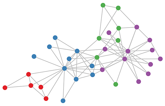
Karate club graph, colors denote communities obtained via modularity-based clustering (Brandes et al., 2008).

Let's take a look at how our simple GCN model (see previous section or Kipf & Welling, ICLR 2017) works on a well-known graph dataset: Zachary's karate club network (see Figure above).

We take a 3-layer GCN with randomly initialized weights. Now, even before training the weights, we simply insert the adjacency matrix of the graph and X=IX=I (i.e. the identity matrix, as we don't have any node features) into the model. The 3-layer GCN now performs three propagation steps during the forward pass and effectively convolves the 3rd-order neighborhood of every node (all nodes up to 3 "hops" away). Remarkably, the model produces an embedding of these nodes that closely resembles the community-structure of the graph (see Figure below). Remember that we have initialized the weights completely at random and have not yet performed any training updates (so far)!

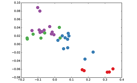
GCN embedding (with random weights) for nodes in the karate club network.

This might seem somewhat surprising. A recent paper on a model called DeepWalk (Perozzi et al., KDD 2014) showed that they can learn a very similar embedding in a complicated unsupervised training procedure. How is it possible to get such an embedding more or less "for free" using our simple untrained GCN model?

We can shed some light on this by interpreting the GCN model as a generalized, differentiable version of the well-known Weisfeiler-Lehman algorithm on graphs. The (1-dimensional) Weisfeiler-Lehman algorithm works as follows3:

For all nodes vi∈Gvi∈G:

• Get features4 {hvj}{hvj} of neighboring nodes {vj}{vj}
• Update node feature hvi←hash(∑jhvj)hvi←hash(∑jhvj), where hash(⋅)hash(⋅) is (ideally) an injective hash function

Repeat for kk steps or until convergence.

In practice, the Weisfeiler-Lehman algorithm assigns a unique set of features for most graphs. This means that every node is assigned a feature that uniquely describes its role in the graph. Exceptions are highly regular graphs like grids, chains, etc. For most irregular graphs, this feature assignment can be used as a check for graph isomorphism (i.e. whether two graphs are identical, up to a permutation of the nodes).

Going back to our Graph Convolutional layer-wise propagation rule (now in vector form):

 

h(l+1)vi=σ(∑j1cijh(l)vjW(l)),hvi(l+1)=σ(∑j1cijhvj(l)W(l)),

 

where jj indexes the neighboring nodes of vivi. cijcij is a normalization constant for the edge (vi,vj)(vi,vj) which originates from using the symmetrically normalized adjacency matrix D−12AD−12D−12AD−12 in our GCN model. We now see that this propagation rule can be interpreted as a differentiable and parameterized (with W(l)W(l)) variant of the hash function used in the original Weisfeiler-Lehman algorithm. If we now choose an appropriate non-linearity and initialize the random weight matrix such that it is orthogonal (or e.g. using the initialization from Glorot & Bengio, AISTATS 2010), this update rule becomes stable in practice (also thanks to the normalization with cijcij). And we make the remarkable observation that we get meaningful smooth embeddings where we can interpret distance as (dis-)similarity of local graph structures!

GCNs Part IV: Semi-supervised learning

Since everything in our model is differentiable and parameterized, we can add some labels, train the model and observe how the embeddings react. We can use the semi-supervised learning algorithm for GCNs introduced in Kipf & Welling (ICLR 2017). We simply label one node per class/community (highlighted nodes in the video below) and start training for a couple of iterations5:

Semi-supervised classification with GCNs: Latent space dynamics for 300 training iterations with a single label per class. Labeled nodes are highlighted.

Note that the model directly produces a 2-dimensional latent space which we can immediately visualize. We observe that the 3-layer GCN model manages to linearly separate the communities, given only one labeled example per class. This is a somewhat remarkable result, given that the model received no feature description of the nodes. At the same time, initial node features could be provided, which is exactly what we do in the experiments described in our paper (Kipf & Welling, ICLR 2017) to achieve state-of-the-art classification results on a number of graph datasets.

Conclusion

Research on this topic is just getting started. The past several months have seen exciting developments, but we have probably only scratched the surface of these types of models so far. It remains to be seen how neural networks on graphs can be further taylored to specific types of problems, like, e.g., learning on directed or relational graphs, and how one can use learned graph embeddings for further tasks down the line, etc. This list is by no means exhaustive and I expect further interesting applications and extensions to pop up in the near future. Let me know in the comments below if you have some exciting ideas or questions to share!

THANKS TO THE FOLLOWING PEOPLE:

Max Welling, Taco Cohen, Chris Louizos and Karen Ullrich (for many discussions and feedback both on the paper and this blog post). Also I'd like to thank Ferenc Huszar for highlighting some drawbacks of these kinds of models.

A NOTE ON COMPLETENESS

This blog post constitutes by no means an exhaustive review of the field of neural networks on graphs. I have left out a number of both recent and older papers to make this post more readable and to give it a coherent story line. The papers that I mentioned here will nonetheless serve as a good start if you want to dive deeper into this topic and get a complete overview of what is around and what has been tried so far.

CITATION

If you want to use some of this in your own work, you can cite our paper on Graph Convolutional Networks:

@article{kipf2016semi,
  title={Semi-Supervised Classification with Graph Convolutional Networks},
  author={Kipf, Thomas N and Welling, Max},
  journal={arXiv preprint arXiv:1609.02907},
  year={2016}
}

SOURCE CODE

We have released the code for Graph Convolutional Networks on GitHub: https://github.com/tkipf/gcn.

You can follow me on Twitter for future updates.

README.md

Graph Convolutional Networks

This is a TensorFlow implementation of Graph Convolutional Networks for the task of (semi-supervised) classification of nodes in a graph, as described in our paper:

Thomas N. Kipf, Max Welling, Semi-Supervised Classification with Graph Convolutional Networks (ICLR 2017)

For a high-level explanation, have a look at our blog post:

Thomas Kipf, Graph Convolutional Networks (2016)

Installation

python setup.py install

Requirements

• tensorflow (>0.12)
• networkx

Run the demo

cd gcn
python train.py

Data

In order to use your own data, you have to provide

• an N by N adjacency matrix (N is the number of nodes),
• an N by D feature matrix (D is the number of features per node), and
• an N by E binary label matrix (E is the number of classes).

Have a look at the load_data() function in utils.py for an example.

In this example, we load citation network data (Cora, Citeseer or Pubmed). The original datasets can be found here: http://www.cs.umd.edu/~sen/lbc-proj/LBC.html. In our version (see data folder) we use dataset splits provided by https://github.com/kimiyoung/planetoid (Zhilin Yang, William W. Cohen, Ruslan Salakhutdinov, Revisiting Semi-Supervised Learning with Graph Embeddings, ICML 2016).

You can specify a dataset as follows:

python train.py --dataset citeseer

(or by editing train.py)

Models

You can choose between the following models:

• gcn: Graph convolutional network (Thomas N. Kipf, Max Welling, Semi-Supervised Classification with Graph Convolutional Networks, 2016)
• gcn_cheby: Chebyshev polynomial version of graph convolutional network as described in (Michaël Defferrard, Xavier Bresson, Pierre Vandergheynst, Convolutional Neural Networks on Graphs with Fast Localized Spectral Filtering, NIPS 2016)
• dense: Basic multi-layer perceptron that supports sparse inputs

Graph classification

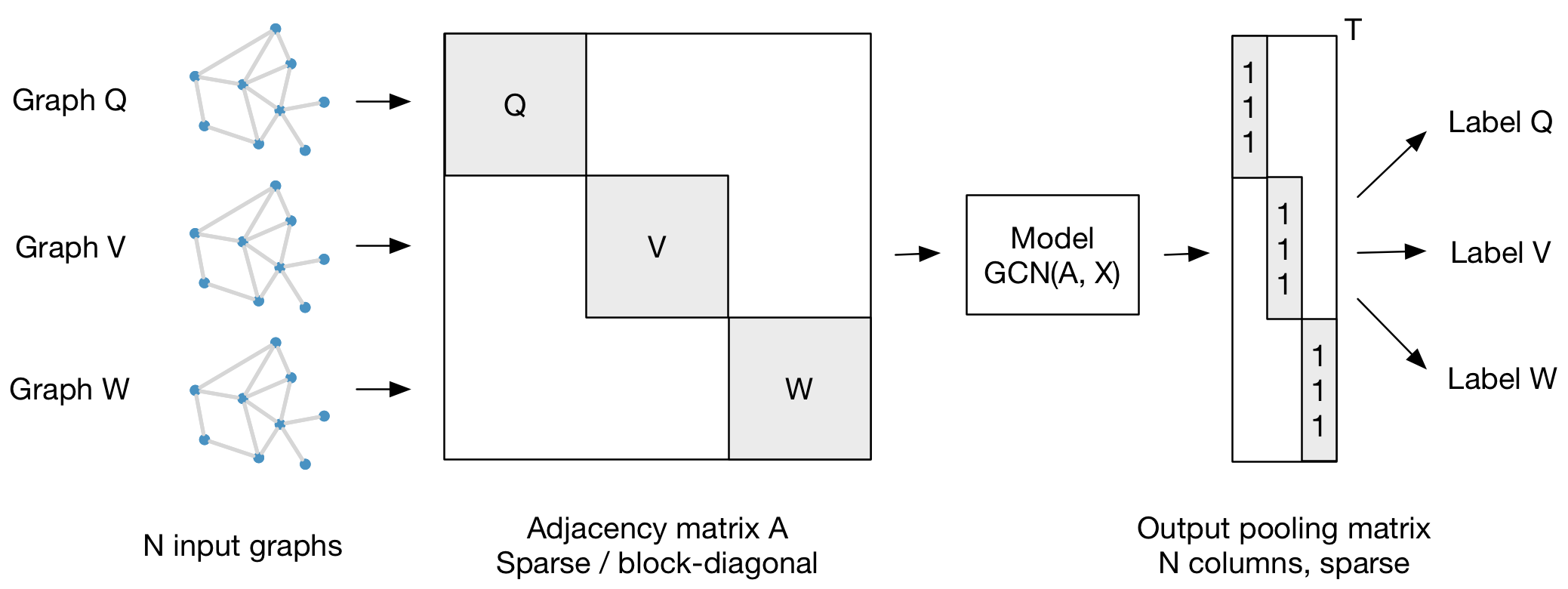
Our framework also supports batch-wise classification of multiple graph instances (of potentially different size) with an adjacency matrix each. It is best to concatenate respective feature matrices and build a (sparse) block-diagonal matrix where each block corresponds to the adjacency matrix of one graph instance. For pooling (in case of graph-level outputs as opposed to node-level outputs) it is best to specify a simple pooling matrix that collects features from their respective graph instances, as illustrated below: