Matplotlib画图常用命令

1. 后处理Epoch结果：代码及图

+ View Code?

1 2 3 4 5 6 7 8 9 10 11 12 13 14 15 16 17 18 19 20 21 22 23 24 25 26 27 28 29 30 31 32 33 34 35 36 37 38 39 40 41 42 43 44 45 46 47 48 49 50 51 52 53 54 55 56 57 58 59 60 61 62 63 64 65 66 67 68 69 70 71 72 73 74 75 76 77

import sdf_helper as sh import numpy as np import matplotlib.pyplot as plt from matplotlib.ticker import MultipleLocator as ml from matplotlib.ticker import ScalarFormatter as sf import matplotlib.ticker as ticker import matplotlib.cm as cm dataname='./0005.sdf' i=500 print(type(i)) print(dataname) data=sh.getdata(dataname) sh.list_variables(data) y=np.linspace(-20,20,400) x=np.linspace(-20,20,400) z=np.linspace(-40,40,800) # X,Y=np.meshgrid(x,y) Y,Z=np.meshgrid(z,y) Ex = ex[:,:,:] Ey = ey[:,:,:] Ez = ez[:,:,:] # fig, ax = plt.subplots() # q = ax.quiver(X, Y, Ex, Ey, color="C1") # #scale_units='xy', scale=5, width=.015 # ax.set_title(r"t=50 laser periods, x=20 $\lambda$") # ax.set_aspect(1.0) # ax.set(xlim=(-15, 15), ylim=(-15, 15)) # fig.savefig('t=3.png',dpi=1000) # plt.show() # #  Plot 1 # vector figure of less points # sEx = np.zeros((40,40)) # sEy = np.zeros((40,40)) # for i in range(1,40): #     for j in range(1,40): #         sEx[i,j] = Ex[i*5*2,j*5*2] #         sEy[i,j] = Ey[i*5*2,j*5*2] # fig, ax = plt.subplots() # q = ax.quiver(sEx, sEy, color="C1") # #scale_units='xy', scale=5, width=.015 # ax.set_title(r"E(x,y) at t=50 laser periods, z=20 $\lambda$") # ax.set_aspect(1.0) # ax.set_xlabel(r"$x [\lambda]$") # ax.set_ylabel(r"$y [\lambda]$") # fig.savefig('t=5small.png',dpi=1000) # plt.show() # # Plot 1 # Density distribution 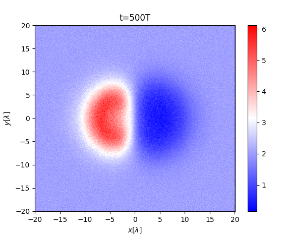n=data.Derived_Number_Density n0=8.9285e27*0.01 fig, ax = plt.subplots() plt.pcolor(Y,Z,n.data[250,:,:]/n0,cmap='bwr') # # plt.colorbar(label="Plasma density", orientation="vertical") titlename="t=" "%d" "T" % i ax.set_title(titlename) ax.set_xlabel(r"$x [\lambda]$") ax.set_ylabel(r"$y [\lambda]$") plt.colorbar() filename1='density at x=x_center" "%d" ".png'  % i fig.savefig(filename1) plt.show() # plot 2 # Laser intensity I=Ex**2+Ey**2 fig,ax=plt.subplots() plt.pcolor(Y,Z,I[200,:,:],cmap='bwr') plt.colorbar() ax.set_xlabel(r"$y [\lambda]$") ax.set_ylabel(r"$z [\lambda]$") titlename="t=" "%d" "T" % i ax.set_title(titlename) # plt.colorbar(label="Laser Intensity", orientation="vertical") filename2="laserIntensity-yz" "%d" ".png" % i fig.savefig(filename2) plt.show()