for large number of missing value imputation in R

using the package “MICE”

install.packages('mice')
library('mice')
pMiss <- function(x){sum(is.na(x))/length(x)}

apply(AFE_psi[,c(12:70)], 1, pMiss)
apply(AFE_psi[,c(12:70)], 2, pMiss)
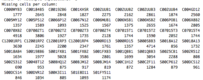
md.pattern(AFE_psi[,c(12:70)])
install.packages('VIM')
library('VIM')
aggr_plot <- aggr(AFE_psi[c(1:20),c(12:70)], col=c('navyblue','red'),
numbers=TRUE,
sortVars=TRUE,
labels=names(AFE_psi[c(1:20),c(12:70)]),
cex.axis=.9,
gap=3,
ylab=c("AFE_data_missing_value_histgram","modes"))
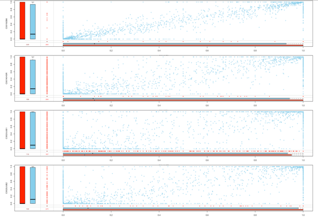
marginplot(AFE_psi[,c(16,17)])###2-2samples_box_plot
tempData <- mice(AFE_psi[,c(12:70)],m=5,maxit=6,meth='pmm',seed=600)

summary(tempData)

可以看到我的59个样本中每个样本的missing value 有多少个

把imputation之后的的dataset用不同的结果数据还原回去

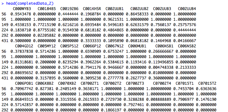
completedData <- complete(tempData,1)##using the first column data to imputate the original dataframe
completedData_2 <- complete(tempData,2)##using the second column data to imputate the original dataframe
查看初始数据和插补数据的分布情况

to compare both distribution to infer the imputated data's fidelity 
library(lattice)
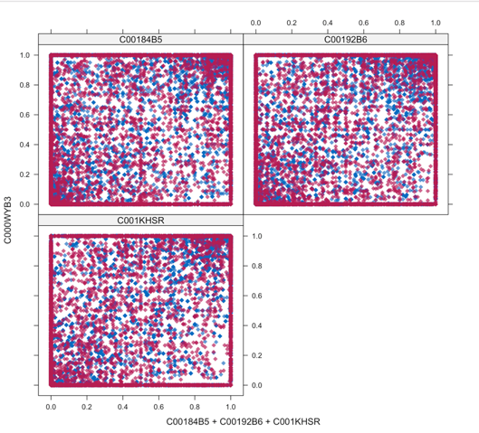
xyplot(tempData,C000WYB3 ~ C00184B5+C00192B6+C001KHSR,pch=18,cex=1)######for the first four samples xyplot
densityplot(tempData)
stripplot(tempData, pch = 20, cex = 1.2)

 前五个样本之间的缺失值存在或者不存在的情况之下，boxplot的分布情况，越一致数据越不受缺失值的影响。

前四个样本之间imputation data 之前之后的fitting situation，洋红色代表imputation之后的data蓝色的代表的是直接observed的data

最后用第二列数据做还原的原始data frame如下：

 

######this chapter mainly using the method of imputationpr——edictive mean matching method，and mice package in R