线性模型之四:逻辑回归
一、问题描述
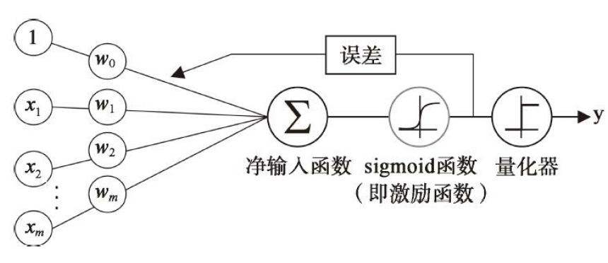
前面我们讨论了使用线性模型进行回归学习,但是要做分类任务怎么办?只需要找一个单调可微函数将任务分类的真实标记 y 与线性回归模型的预测值联系起来。
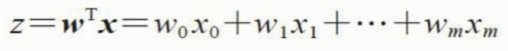
考虑二分类任务,其输出应该是 y 属于[0, 1]。而线性回归模型产生的预测值 z = wx+b是实值。于是我们考虑将 z 转换到 0 / 1值。
二、对数几率回归
最理想的将实值转换为[0, 1]区间的是单位阶跃函数。
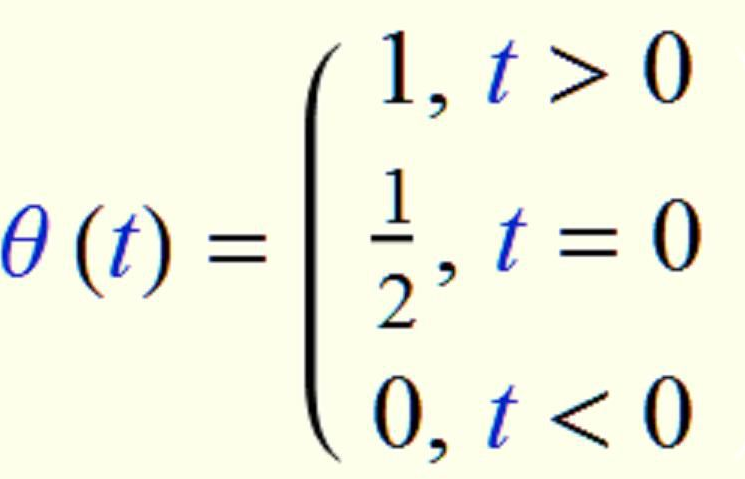
但是这个函数不连续,所以要考虑其他的函数。
先介绍一下几率回归。它指的是特定事件发生的几率。用数学公式: p/(1-p)
其中p为正事件发生的概率,指的是我们关注事件发生的概率。更进一步,可以定义logit函数,对数几率,
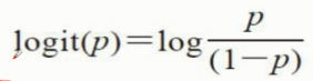
logit函数输入范围介于区间[0, 1], 它能将输入转换到整个实数范围内。而我们之前考虑的函数映射将实值转换为[0, 1],所以考虑logit的反函数。
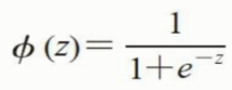
此处,p(y=1|x)是在给定特征x的条件下,某一个样本属于类别1的条件概率。它是logit函数的反函数,也称作logistic函数,也称为sigmoid函数。
这里,z 作为输入
sigmoid函数的图形
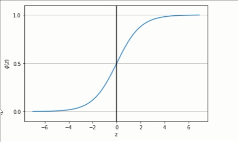
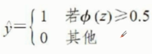
当s函数输入大于0时,s函数的输出大于0.5,反之则小于0.5。
sigmoid函数的输出值 p 介于[0, 1]之间,表示某个事件发生的概率。
三、代价函数
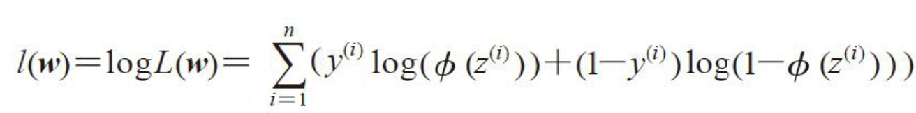
为了推导出逻辑回归的代价函数,需要先定义一个最大似然函数L

对于二分类问题,y只能有两个值1 和 0。
![]() 为s函数的输出值,用来表示概率的大小。如果y为1时,预测的概率值为
为s函数的输出值,用来表示概率的大小。如果y为1时,预测的概率值为![]() ,我们希望
,我们希望![]() 尽可能大。
尽可能大。
如果y为0,预测的概率值为![]() ,我们则希望
,我们则希望![]() 尽可能大。
尽可能大。
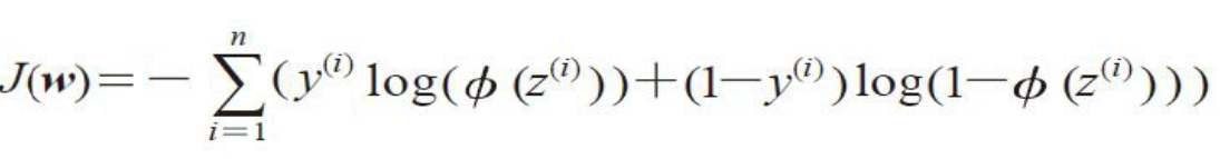
那么写成一个表达式,![]() 。我们希望这个表达式的值尽可能最大。
。我们希望这个表达式的值尽可能最大。
我们的目标是使用已知的N个样本,使得这个L的概率值最大。由于连乘不容易处理,可以使用取对数的方法,转化为连加。
对数似然函数可以更容易求导。然后加上负号,可以使用梯度下降算法求解函数的最小值了。
四、正则化

sklearn 库中,LogisticRegression类,参数C是正则化系数的倒数

代码示例:
LogisticRegressionGD.py
import numpy as np

class LogisticRegressionGD(object):
    """Logistic Regression Classifier using gradient descent.

    Parameters
    ------------
    eta : float
      Learning rate (between 0.0 and 1.0)
    n_iter : int
      Passes over the training dataset.
    random_state : int
      Random number generator seed for random weight
      initialization.

    Attributes
    -----------
    w_ : 1d-array
      Weights after fitting.
    cost_ : list
      Sum-of-squares cost function value in each epoch.

    """
    def __init__(self, eta=0.05, n_iter=100, random_state=1):
        self.eta = eta
        self.n_iter = n_iter
        self.random_state = random_state

    def fit(self, X, y):
        """ Fit training data.

        Parameters
        ----------
        X : {array-like}, shape = [n_samples, n_features]
          Training vectors, where n_samples is the number of samples and
          n_features is the number of features.
        y : array-like, shape = [n_samples]
          Target values.

        Returns
        -------
        self : object

        """
        rgen = np.random.RandomState(self.random_state)
        self.w = rgen.normal(loc = 0.0, scale=0.01, size = 1+X.shape[1])
        self.cost = []

        for i in range(self.n_iter):
            output = self.activation(self.net_input(X))
            error = y - output
            self.w[1:] = self.w[1:] + self.eta * X.T.dot(error)
            self.w[0] = self.w[0] + self.eta * np.sum(error)
            #each_cost = -np.sum((y * np.log(output)+(1-y) * np.log(1-output)))
            each_cost = -y.dot(np.log(output)) - (1-y).dot(np.log(1-output))
            self.cost.append(each_cost)
        return self

    def net_input(self, X):
        """Calculate net input"""
        return np.dot(X, self.w[1:]) + self.w[0]

    def activation(self, z):
        """Compute logistic sigmoid activation"""
        return 1 / (1+ np.exp(-z))

    def predict(self, X):
        """Return class label after unit step"""
        return np.where(self.net_input(X) >= 0, 1, 0)
        # equivalent to:
        # return np.where(self.activation(self.net_input(X)) >= 0.5, 1, 0)
testLogisticRegression.py
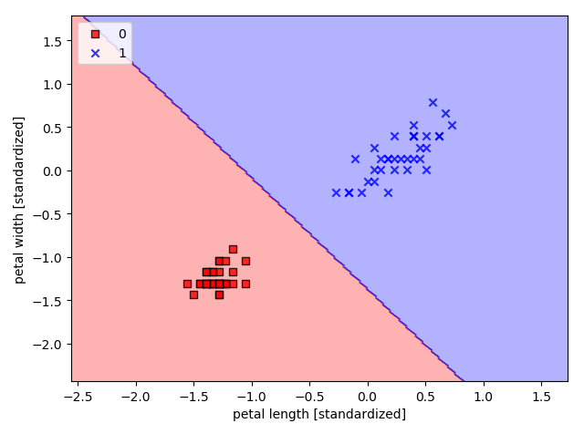
import matplotlib.pylab as plt
import numpy as np
from LogisticRegressionGD import LogisticRegressionGD
from sklearn import datasets

iris_data = datasets.load_iris()
x = iris_data.data[:, [2, 3]]
y = iris_data.target

#print('Class Labels:', np.lib.arraysetops.unique(y))

from sklearn.model_selection import train_test_split

X_train, X_test, y_train, y_test  = train_test_split(
    x, y, test_size=0.3, random_state=1, stratify=y)

#print('labels counts in y:', np.bincount(y))
#print('labels counts in y_train:', np.bincount(y_train))
#print('labels counts in y_test:', np.bincount(y_test))

from sklearn.preprocessing import StandardScaler
sc = StandardScaler()
sc.fit(X_train)
X_train_std = sc.transform(X_train)
X_test_std = sc.transform(X_test)

# In[]:
from matplotlib.colors import ListedColormap
import matplotlib.pyplot as plt
# 分类决策区域函数
# 注意,这个cell也必须run,把画图函数载入进来,否则后面无法调用
def plot_decision_regions(X, y, classifier, test_idx=None, resolution=0.02):

    # setup marker generator and color map
    markers = ('s', 'x', 'o', '^', 'v')
    colors = ('red', 'blue', 'lightgreen', 'gray', 'cyan')
    cmap = ListedColormap(colors[:len(np.unique(y))])

    # plot the decision surface
    x1_min, x1_max = X[:, 0].min() - 1, X[:, 0].max() + 1
    x2_min, x2_max = X[:, 1].min() - 1, X[:, 1].max() + 1
    xx1, xx2 = np.meshgrid(np.arange(x1_min, x1_max, resolution),
                           np.arange(x2_min, x2_max, resolution))
    Z = classifier.predict(np.array([xx1.ravel(), xx2.ravel()]).T)
    Z = Z.reshape(xx1.shape)
    plt.contourf(xx1, xx2, Z, alpha=0.3, cmap=cmap)
    plt.xlim(xx1.min(), xx1.max())
    plt.ylim(xx2.min(), xx2.max())

    for idx, cl in enumerate(np.unique(y)):
        plt.scatter(x=X[y == cl, 0],
                    y=X[y == cl, 1],
                    alpha=0.8,
                    c=colors[idx],
                    marker=markers[idx],
                    label=cl,
                    edgecolor='black')

    # highlight test samples
    if test_idx:
        # plot all samples
        X_test, y_test = X[test_idx, :], y[test_idx]

        plt.scatter(X_test[:, 0],
                    X_test[:, 1],
                    c='',
                    edgecolor='black',
                    alpha=1.0,
                    linewidth=1,
                    marker='o',
                    s=100,
                    label='test set')

X_train_01_subset = X_train_std[(y_train == 0) | (y_train == 1)]
y_train_01_subset = y_train[(y_train == 0) | (y_train == 1)]

lrgd = LogisticRegressionGD(eta=0.05, n_iter=1000, random_state=1)
print(X_train_01_subset.shape)
print(y_train_01_subset.shape)
lrgd.fit(X_train_01_subset, y_train_01_subset)
plot_decision_regions(X_train_01_subset, y_train_01_subset,
                      classifier=lrgd)
plt.xlabel('petal length [standardized]')
plt.ylabel('petal width [standardized]')
plt.legend(loc='upper left')

plt.tight_layout()
plt.show()
输出示例

 浙公网安备 33010602011771号