Machine Learning Week_7 Support Vector Machines

目录

• 1 Large Margin Classification
  • 1.1 Optimization Objective
    • 1.1 Logistic Regresson
    • 1.2 Cost
    • 1.3 Suppport vector machine
    • 1.4 SVM hypothesis
  • 1.2 Large Margin Intuition
  • 1.3 Mathematics Behind Large Margin Classification
• 2 Kernels
  • 2.1 Kernels I
    • 2.1 kernel:
  • 2.2 Kernels II
    • 2.2.1 SVM with kernels
    • 2.2.2 SVM pramaters
• 3 SVMS In Practice
  • 3.1 Using An SVM
  • 3.2 Other choices of kernel
  • 3.3 implatation
  • 3.4 Multi-class classification
  • 3.5 LR VS SVM

1 Large Margin Classification

1.1 Optimization Objective

By now, you've seen a range of difference learning algorithms.

With supervised learning, the performance of many supervised learning algorithms will be pretty similar, and what matters less often will be whether you use learning algorithm a or learning algorithm b, but what matters more will often be things like the amount of data you create these algorithms on, as well as your skill in applying these algorithms.

Things like your choice of the features you design to give to the learning algorithms, and how you choose the regularization parameter, and things like that. But, there's one more algorithm that is very powerful and is very widely used both within industry and academia, and that's called the support vector machine. And compared to both logistic regression and neural networks, the Support Vector Machine, or SVM sometimes gives a cleaner, and sometimes more powerful way of learning complex non-linear functions.

And so let's take the next videos to talk about that. Later in this course, I will do a quick survey of a range of different supervise algorithms just as a very briefly describe them. But the support vector machine, given its popularity and how powerful it is, this will be the last of the supervisory algorithms that I'll spend a significant amount of time on in this course as with our development other learning algorithms, we're gonna start by talking about the optimization objective.

So, let's get started on this algorithm.

In order to describe the support vector machine, I'm actually going to start with logistic regression, and show how we can modify it a bit, and get what is essentially the support vector machine. So in logistic regression, we have our familiar form of the hypothesis there and the sigmoid activation function.

1.1 Logistic Regresson

$$\begin{array}{rl}& h_{\theta }(x)=g({\theta }^{T}x)\\ \\ & z={\theta }^{T}x\\ & g(z)={\displaystyle \frac{1}{1+e^{-z}}}\end{array}$$

$$\begin{array}{rl}& {\theta }^{T}x\ge 0\Rightarrow y=1\\ & {\theta }^{T}x<0\Rightarrow y=0\end{array}$$

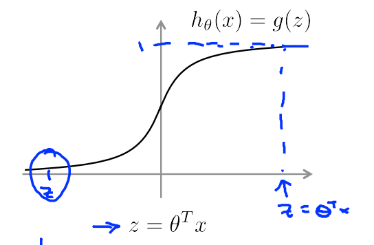
if y=1, we want $h_{\theta }(x)\approx 1$，${\theta }^{T}x\gg 0$
if y=0, we want $h_{\theta }(x)\approx 0$，${\theta }^{T}x\ll 0$

1.2 Cost

Cost of example:

$$-y\log (h_{\theta }(x))-(1-y)\log (1-h_{\theta }(x))$$

我们将逻辑回归的代价函数图像可以修正为如下图所示，从而得出支持向量机的代价函数。

1.3 Suppport vector machine

logistic regression:

$$mi{n}_{\theta }\frac{1}{m}\sum _{i=1}^m[y^{(i)}(-\log (h_{\theta }(x^{(i)})))+(1-y^{(i)})(-\log (1-h_{\theta }(x^{(i)})))]+\frac{\lambda }{2m}\sum _{j=1}^n{\theta }_j^2$$

Support machine:

$$mi{n}_{\theta }C\sum _{i=1}^m[y^{(i)}cost({\theta }^T{x}^{(i)})+(1-y^{(i)})cost({\theta }^T{x}^{(i)})]+\frac{1}{2}\sum _{j=1}^n{\theta }_j^2$$

两个式子可以简化；

$$A+\lambda B$$

$$CA+B$$

有一个技巧是 C 可以看作 $C=\frac{1}{\lambda }$

1.4 SVM hypothesis

$$\begin{array}{rl}& {\theta }^{T}x\ge 0\Rightarrow y=1\\ & {\theta }^{T}x<0\Rightarrow y=0\end{array}$$

Finally unlike logistic regression, the support vector machine doesn't output the probability is that what we have is we have this cost function, that we minimize to get the parameter's data, and what a support vector machine does is it just makes a prediction of y being equal to one or zero, directly. So the hypothesis will predict one if theta transpose x is greater or equal to zero, and it will predict zero otherwise and so having learned the parameters theta, this is the form of the hypothesis for the support vector machine. So that was a mathematical definition of what a support vector machine does. In the next few videos, let's try to get back to intuition about what this optimization objective leads to and whether the source of the hypotheses SVM will learn and we'll also talk about how to modify this just a little bit to the complex nonlinear functions.

1.2 Large Margin Intuition

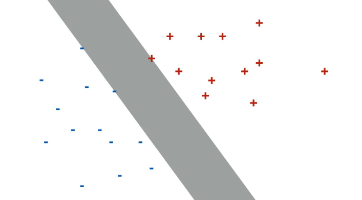
Sometimes people talk about support vector machines, as large margin classifiers.

SVM可以看作是用一根很宽的小棒子去分类，棒子越宽越好。而LR时用线分，所以有时候得出来的结果并不好。

为了找到这个边界，在逻辑回归中，我们需要 ${\theta }^{T}x\ge 0(w^{T}x+b\ge 0)$. 这里 ${\theta }_0{x}_0=b$ 是偏置项。

一旦确定了 $w$ $b$ 那我们就确定了决策的边界。我们可以看到，一条决策边界就是 $w^{T}x+b=0$, 是一个点积。点积等于0，两个向量垂直。$b$ 控制这边界的偏移。$w$ 控制这边界斜率。

在SVM中，也是同样的方法，但是 ${\theta }^{T}x\ge 1(w^{T}x+b\ge 1)$

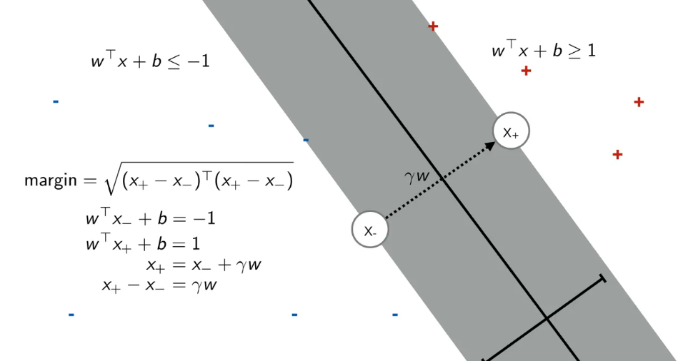
通过一番转换，带入。

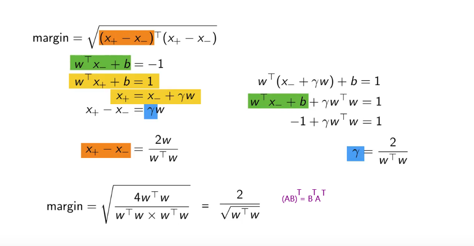
我们想要 Margin 最大，就需要 $\sqrt{w^{T}w}$ 最小。这也是SVM代价函数里 $\frac{1}{2}\sum _{j=1}^n{\theta }_j^2$, 有无根号没有关系。

如果 $y_{+}=1,y_{-}=-1$，上面的两个分界可以写成一个 $y(w^{T}x+b)\ge 1$。

其实课程作业里也将 $y=0$ 变成 $y=-1$ 了.

% svmTarin.m
% [model] = svmTarin(X, Y, C, kernelFunction, tol, max_passes)
% Map 0 to -1
Y(Y==0) = -1;

% ex6.m
% model = svmTrain(X, y, C, @linearKernel, 1e-3, 20);

这确实是一个非常好的思想，可是世界上哪有绝对的间距为2的分类呢。因为不可能恰好用宽为2的棒子分开所有不同的点。这时候我们就要给他来点人性化。说你小子不要太死板。

修正:

$$y(w^{T}x+b)\ge 1-\xi$$

$$\xi \ge 0$$

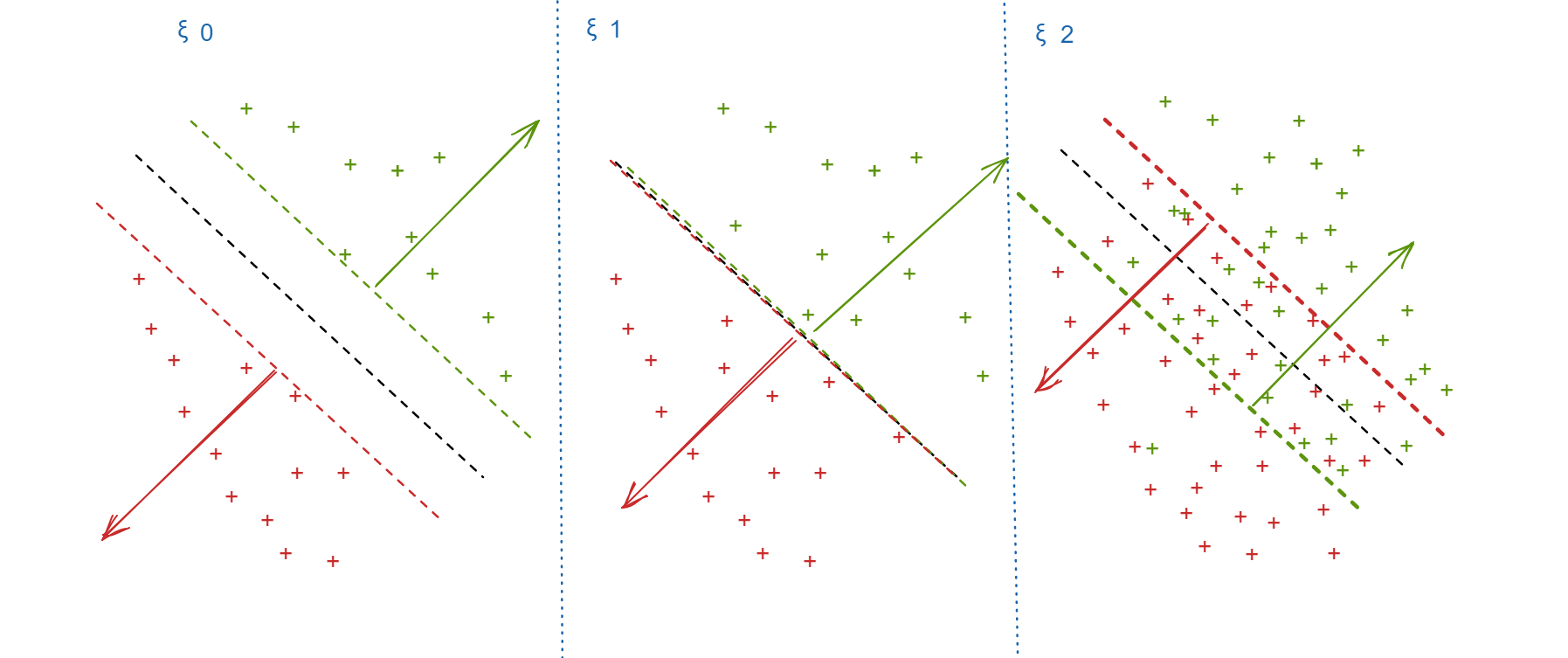
这是C的由来。 我们的目标是

$$min\frac{1}{2}{w}^{T}w+C\xi$$

当C很大时，我们知道这对应者分类的极大准确性和大间隔。而这对应需要很小的 $\xi$, 反之需要很大的 $\xi$，我们可以让部分决策区域重合，来达到一个模糊的软的分类。

1.3 Mathematics Behind Large Margin Classification

In this video, I'd like to tell you a bit about the math behind large margin classification.

This video is optional, so please feel free to skip it. It may also give you better intuition about how the optimization problem of the support vex machine, how that leads to large margin classifiers.

In order to get started, let me first remind you of a couple of properties of what vector inner products look like.

很显然，两个老师的对于SVM的理解不同，但都是正确的。这也告诉我们要从多角度看问题，一个问题肯定有多角度的理解。之前的公式是用的 n 维，现在用的是 n+1 维。

$$\begin{array}{rl}{u}^{T}v& =u_1{v}_1+u_2{v}_2\\ & =p\cdot ||u||\end{array}$$

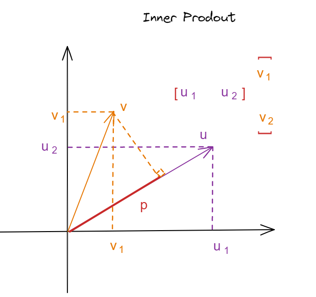
where $p$ is the projection of $v$ into the $u$

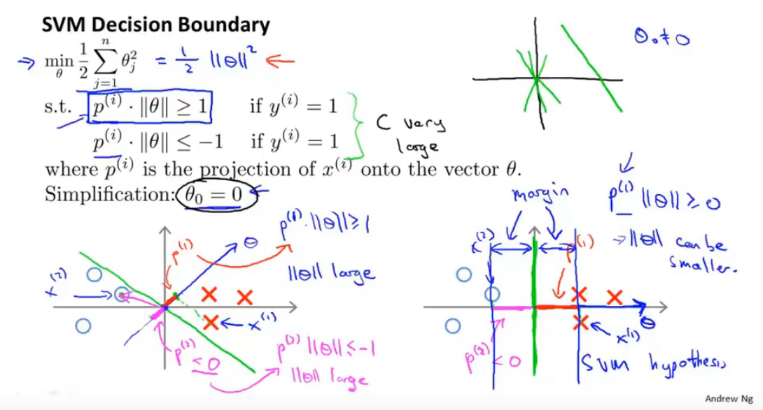
$p$ 是 $x$ 向 $\theta$ 投影的长度，也就是 $x$ 离决策边界的距离。n+1 维的 $\theta$ 垂直于决策边界。

这里有一个问题。

$${\theta }^{T}x=0$$

$$w^{T}x+b=0$$

这两个怎么都垂直于$x$, 当然这两个x的维度不同。$w$ 某种程度上与 $x$ 的斜率有关，不过为什么。形式不一样还都垂直。

其实向量不就是线么？或者说三维的空间里也可以有直线存在，这与二维里的线没什么不同，只是方向多了一点。

2 Kernels

2.1 Kernels I

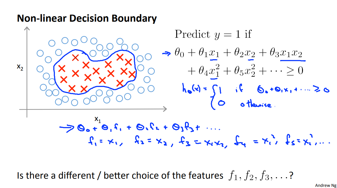
In this video, I'd like to start adapting support vector machines in order to develop complex nonlinear classifiers. The main technique for doing that is something called kernels. Let's see what this kernels are and how to use them.

写到这里，忽然对之前的知识有了一个明悟。以前一直以为线性回归的逻辑回归完全没有太大用处，决策边界很简单。一到了非线性的时候就得上神经网络。

现在才明白，线性回归有什么差的？2维问题它得到一条直线，3维问题它能得到一个平面，4维问题问题它可以得到一个3维的体。如此往复，只要维度高，什么复杂的图形我都可以做出来。这也是为什么400维的手写数字识别，它可以达到90+%的正确率。与神经网络不相上下。

不过当我的维度受限时，非线性的分类可以很好的拟合，例如2维的非线性可以拟合2维的决策边界。高了很多么？不见得。这么说来，当我有2维的数据时，如果2维的线性拟合不出来，简单的我就可以简单的选择出其他的特征，将它的维度变高，那么线性边界的复杂度也会提高。当然也可以用一个神经网络去做。

重要的是，抽象出什么特征向量来。是已有特征的复合，或是创造一个新的变量出来。

下面的高斯核函数，就是低维向高维做映射。

2.1 kernel:

我们先来谈论一下高斯分布，或者说是正态分布。若随机变量服从一个数学期望为$\mu$, 方差为${\sigma }^2$的正态分布，记为$\mathbb{N}(\mu ,{\sigma }^2)$。方差大数据离散，图像就会平缓一点，方差小数据比较集中，图像就会陡峭一点。

$$f(x)=\frac{1}{\sigma \sqrt{2\pi }}exp(-\frac{(x-\mu {)}^2}{2{\sigma }^2})$$

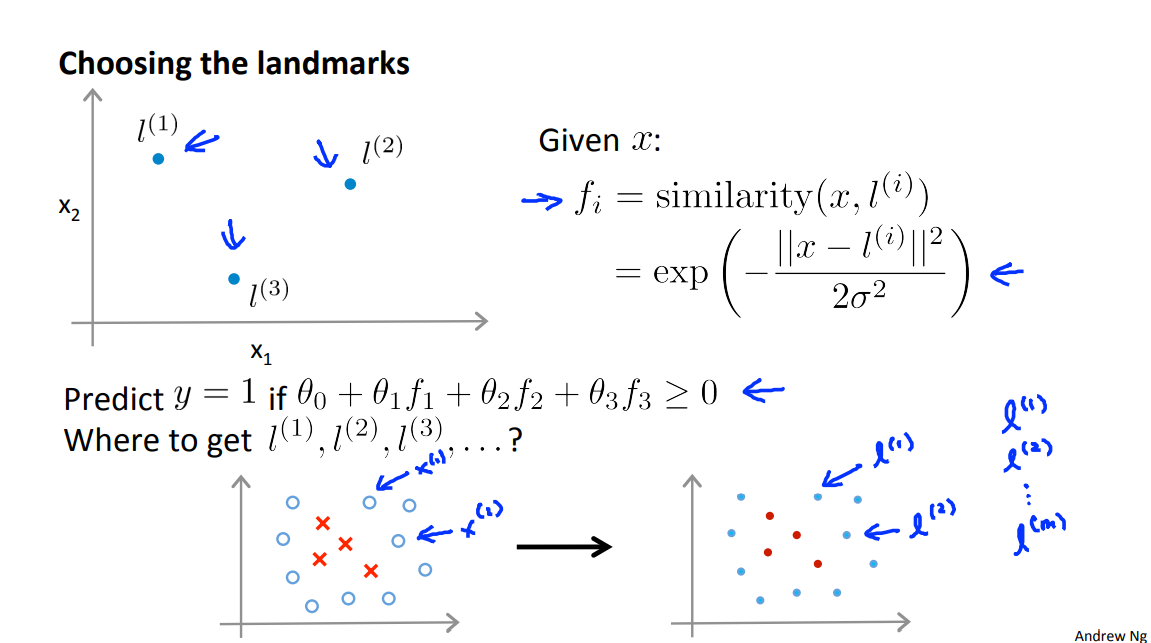
Given x, compute new features $f_1,f_2,f_3...$ depending on proximity to landmarks $l^{(1)},l^{(2)},l^{(3)}...$

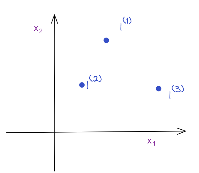
Given x:

$$f_i=\text{similarity}(x,l^{(i)})=exp(-\frac{||x-l^{(i)}|{|}^2}{2{\sigma }^2})$$

这里的$l^{(i)}$ 取数据集中的数据。

if $x\approx l^{(1)}$

$$f_1\approx exp(-\frac{0^2}{2{\sigma }^2})\approx 1$$

if $x$ is far from $l^{(1)}$

$$f_1\approx exp(-\frac{(largenumber{)}^2}{2{\sigma }^2})\approx 1$$

$$l^{(1)}\to f_1,l^{(2)}\to f_2,...,l^{(m)}\to f_m$$

下面是$\sigma$取值的直观理解。

But there are a couple of questions that we haven't answered yet. One is, how do we get these landmarks? How do we choose these landmarks? And another is, what other similarity functions, if any, can we use other than the one we talked about, which is called the Gaussian kernel. In the next video we give answers to these questions and put everything together to show how support vector machines with kernels can be a powerful way to learn complex nonlinear functions.

2.2 Kernels II

In the last video, we started to talk about the kernels idea and how it can be used to define new features for the support vector machine. In this video, I'd like to throw in some of the missing details and, also, say a few words about how to use these ideas in practice. Such as, how they pertain to, for example, the bias variance trade-off in support vector machines.

In the last video, I talked about the process of picking a few landmarks. You know, l1, l2, l3 and that allowed us to define the similarity function also called the kernel or in this example if you have this similarity function this is a Gaussian kernel.

2.2.1 SVM with kernels

Given

$$(x^{(1)},y^{(1)}),(x^{(1)},y^{(1)}),...(x^{(m)},y^{(m)})$$

Choose

$$(l^{(1)}=x^{(1)}),(l^{(2)}=x^{(2)}),...(l^{(m)}=x^{(m)})$$

$$x^{(i)}=x_{m\times 1}^{(i)}=\left[\begin{array}{c}similarity(x,l^{(1)})\\ similarity(x,l^{(2)})\\ ⋮\\ similarity(x,l^{(m)})\end{array}\right]=f^{(i)}add{f}_0^{(i)}=1$$

2.2.2 SVM pramaters

• C
  • large C: lower bias, high variance
  • small C: high bias, lower variance
• $\sigma$
  • large $\sigma$: Feacture f very more smoothly. high bias, lower variance
  • small $\sigma$: Feacture f very less more smoothly. lower bias, high variance

3 SVMS In Practice

3.1 Using An SVM

1. No kernel(linear kernel): when n large, m small

2. Gaussian kernel: when n small, m large。

Note： Do perform feature scaling before using Gaussian kernel.

3.2 Other choices of kernel

Note:Not all similarity functions $similarity(x,l^{(i)})$ make valid kernels.
(Need to satisfy technical condition called “Mercer's Theorem” to make sure 'SVM' packages optimizations run correctly, and do not diverge).

• Polynomial kernel: ....
• More esoteric: String kernel(0), chi-square kernel(1), histgram intersection kernel(2).

数字是老师用过的次数。

3.3 implatation

So just as today, very few of us, or maybe almost essentially none of us would think of writing code ourselves to invert a matrix or take a square root of a number, and so on. We just, you know, call some library function to do that. In the same way, the software for solving the SVM optimization problem is very complex, and there have been researchers that have been doing essentially numerical optimization research for many years. So you come up with good software libraries and good software packages to do this. And then strongly recommend just using one of the highly optimized software libraries rather than trying to implement something yourself. And there are lots of good software libraries out there. The two that I happen to use the most often are the linear SVM but there are really lots of good software libraries for doing this that you know, you can link to many of the major programming languages that you may be using to code up learning algorithm.

Even though you shouldn't be writing your own SVM optimization software, there are a few things you need to do, though. First is to come up with with some choice of the parameter's C. We talked a little bit of the bias/variance properties of this in the earlier video.

Second, you also need to choose the kernel or the similarity function that you want to use. So one choice might be if we decide not to use any kernel.

Note: This is a simplified version of the SMO algorithm for training
%       SVMs. In practice, if you want to train an SVM classifier, we
%       recommend using an optimized package such as:  
%
%           LIBSVM   (http://www.csie.ntu.edu.tw/~cjlin/libsvm/)
%           SVMLight (http://svmlight.joachims.org/)
%

And the idea of no kernel is also called a linear kernel. So if someone says, I use an SVM with a linear kernel, what that means is you know, they use an SVM without using without using a kernel and it was a version of the SVM that just uses theta transpose X.

function sim = gaussianKernel(x1, x2, sigma)
%RBFKERNEL returns a radial basis function kernel between x1 and x2
%   sim = gaussianKernel(x1, x2) returns a gaussian kernel between x1 and x2
%   and returns the value in sim

% Ensure that x1 and x2 are column vectors
x1 = x1(:); x2 = x2(:);

% You need to return the following variables correctly.
sim = 0;

% ====================== YOUR CODE HERE ======================
% Instructions: Fill in this function to return the similarity between x1
%               and x2 computed using a Gaussian kernel with bandwidth
%               sigma
%
%

sim = exp(-sum((x1 - x2).^ 2) / (2 * sigma.^2 ));

% =============================================================
end

这个感觉更像是多项式的核。

function sim = linearKernel(x1, x2)
%LINEARKERNEL returns a linear kernel between x1 and x2
%   sim = linearKernel(x1, x2) returns a linear kernel between x1 and x2
%   and returns the value in sim

% Ensure that x1 and x2 are column vectors
x1 = x1(:); x2 = x2(:);

% Compute the kernel
sim = x1' * x2;  % dot product

end

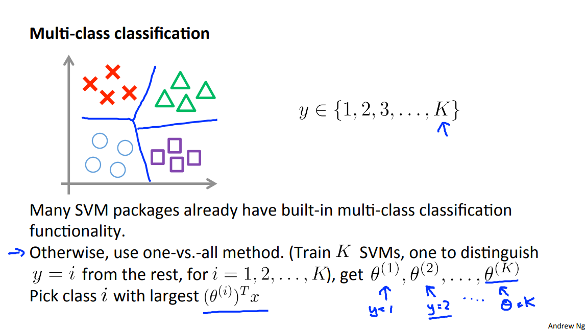
3.4 Multi-class classification

3.5 LR VS SVM

So, when should we use one algorithm versus the other?

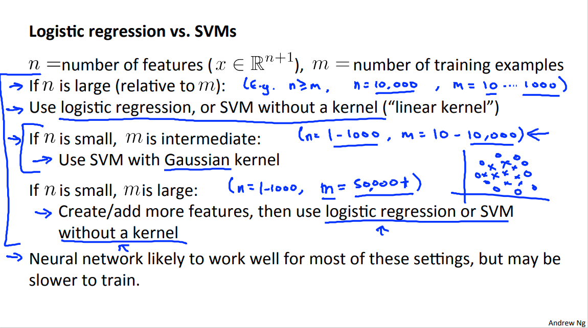
Well, if n is larger relative to your training set size, so for example,

if you take a business with a number of features this is much larger than m and this might be, for example, if you have a text classification problem, where you know, the dimension of the feature vector is I don't know, maybe, 10 thousand.

And if your training set size is maybe 10 you know, maybe, up to 1000. So, imagine a spam classification problem, where email spam, where you have 10,000 features corresponding to 10,000 words but you have, you know, maybe 10 training examples or maybe up to 1,000 examples.

So if n is large relative to m, then what I would usually do is use logistic regression or use it as the m without a kernel or use it with a linear kernel. Because, if you have so many features with smaller training sets, you know, a linear function will probably do fine, and you don't have really enough data to fit a very complicated nonlinear function. Now if is n is small and m is intermediate what I mean by this is n is maybe anywhere from 1 - 1000, 1 would be very small. But maybe up to 1000 features and if the number of training examples is maybe anywhere from 10, you know, 10 to maybe up to 10,000 examples. Maybe up to 50,000 examples. If m is pretty big like maybe 10,000 but not a million. Right? So if m is an intermediate size then often an SVM with a linear kernel will work well. We talked about this early as well, with the one concrete example, this would be if you have a two dimensional training set. So, if n is equal to 2 where you have, you know, drawing in a pretty large number of training examples.

So Gaussian kernel will do a pretty good job separating positive and negative classes.

One third setting that's of interest is if n is small but m is large. So if n is you know, again maybe 1 to 1000, could be larger. But if m was, maybe 50,000 and greater to millions.

So, 50,000, a 100,000, million, trillion.

You have very very large training set sizes, right.

So if this is the case, then a SVM of the Gaussian Kernel will be somewhat slow to run. Today's SVM packages, if you're using a Gaussian Kernel, tend to struggle a bit. If you have, you know, maybe 50 thousands okay, but if you have a million training examples, maybe or even a 100,000 with a massive value of m. Today's SVM packages are very good, but they can still struggle a little bit when you have a massive, massive trainings that size when using a Gaussian Kernel.

So in that case, what I would usually do is try to just manually create have more features and then use logistic regression or an SVM without the Kernel.

And in case you look at this slide and you see logistic regression or SVM without a kernel. In both of these places, I kind of paired them together. There's a reason for that, is that logistic regression and SVM without the kernel, those are really pretty similar algorithms and, you know, either logistic regression or SVM without a kernel will usually do pretty similar things and give pretty similar performance, but depending on your implementational details, one may be more efficient than the other. But, where one of these algorithms applies, logistic regression where SVM without a kernel, the other one is to likely to work pretty well as well. But along with the power of the SVM is when you use different kernels to learn complex nonlinear functions. And this regime, you know, when you have maybe up to 10,000 examples, maybe up to 50,000. And your number of features, this is reasonably large. That's a very common regime and maybe that's a regime where a support vector machine with a kernel kernel will shine. You can do things that are much harder to do that will need logistic regression. And finally, where do neural networks fit in? Well for all of these problems, for all of these different regimes, a well designed neural network is likely to work well as well.

The one disadvantage, or the one reason that might not sometimes use the neural network is that, for some of these problems, the neural network might be slow to train. But if you have a very good SVM implementation package, that could run faster, quite a bit faster than your neural network.

And, although we didn't show this earlier, it turns out that the optimization problem that the SVM has is a convex optimization problem and so the good SVM optimization software packages will always find the global minimum or something close to it. And so for the SVM you don't need to worry about local optima.

In practice local optima aren't a huge problem for neural networks but they all solve, so this is one less thing to worry about if you're using an SVM.

And depending on your problem, the neural network may be slower, especially in this sort of regime than the SVM. In case the guidelines they gave here, seem a little bit vague and if you're looking at some problems, you know, the guidelines are a bit vague, I'm still not entirely sure, should I use this algorithm or that algorithm, that's actually okay.

When I face a machine learning problem, you know, sometimes its actually just not clear whether that's the best algorithm to use, but as you saw in the earlier videos, really, you know, the algorithm does matter, but what often matters even more is things like, how much data do you have. And how skilled are you, how good are you at doing error analysis and debugging learning algorithms, figuring out how to design new features and figuring out what other features to give you learning algorithms and so on. And often those things will matter more than what you are using logistic regression or an SVM. But having said that, the SVM is still widely perceived as one of the most powerful learning algorithms, and there is this regime of when there's a very effective way to learn complex non linear functions.

And so I actually, together with logistic regressions, neural networks, SVM's, using those to speed learning algorithms you're I think very well positioned to build state of the art you know, machine learning systems for a wide region for applications and this is another very powerful tool to have in your arsenal. One that is used all over the place in Silicon Valley, or in industry and in the Academia, to build many high performance machine learning system.