Machine Learning Week_4 Neural Networks: Representation

目录

• 0 Neural Networks: Representation
• 1 Motivations
  • 1.1 Non-linear Hypotheses
  • 1.2 Neurons and the Brain
• 2 Neural Networks
  • 2.1 Model Representation I
  • 2.2 Model Representation II
• 3 Applications
  • 3.1 Examples and Intuitions I
  • 3.2 Examples and Intuitions II
  • 3.3 Multiclass Classification

0 Neural Networks: Representation

Welcome to week 4!

This week, we are covering neural networks. Neural networks is a model inspired by how the brain works. It is widely used today in many applications: when your phone interprets and understand your voice commands, it is likely that a neural network is helping to understand your speech; when you cash a check, the machines that automatically read the digits also use neural networks. --by Andrew NG

1 Motivations

1.1 Non-linear Hypotheses

In this and in the next set of videos, I'd like to tell you about a learning algorithm called a Neural Network.We're going to first talk about the representation and then in the next set of videos talk about learning algorithms for it.

Neutral networks is actually a pretty old idea, but had fallen out of favor for a while. But today, it is the state of the art technique for many different machine learning problems.

So why do we need yet another learning algorithm? We already have linear regression and we have logistic regression, so why do we need, you know, neural networks?

In order to motivate the discussion of neural networks, let me start by showing you a few examples of machine learning problems where we need to learn complex non-linear hypotheses.

Consider a supervised learning classification problem where you have a training set like this.

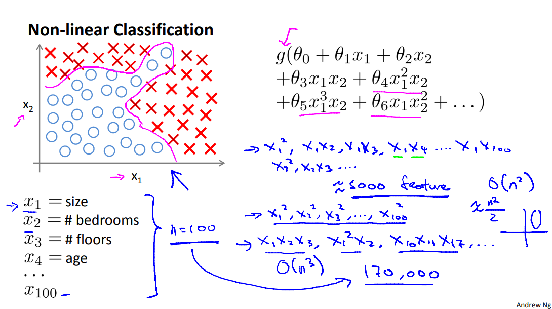
If you want to apply logistic regression to this problem, one thing you could do is apply logistic regression with a lot of nonlinear features like that. So here, g as usual is the sigmoid function, and we can include lots of polynomial terms like these. And, if you include enough polynomial terms then, you know, maybe you can get a hypotheses that separates the positive and negative examples. This particular method works well when you have only, say, two features - x1 and x2 - because you can then include all those polynomial terms of x1 and x2. But for many interesting machine learning problems would have a lot more features than just two.

We've been talking for a while about housing prediction, and suppose you have a housing classification problem rather than a regression problem, like maybe if you have different features of a house, and you want to predict what are the odds that your house will be sold within the next six months, so that will be a classification problem.

And as we saw we can come up with quite a lot of features, maybe a hundred different features of different houses.

For a problem like this, if you were to include all the quadratic terms, all of these, even all of the quadratic that is the second or the polynomial terms, there would be a lot of them. There would be terms like x1 squared, x1x2, x1x3, you know, x1x4 up to x1x100 and then you have x2 squared, x2x3 and so on. And if you include just the second order terms, that is, the terms that are a product of, you know, two of these terms, x1 times x1 and so on, then, for the case of n equals 100, you end up with about five thousand features.

And, asymptotically, the number of quadratic features grows roughly as order n squared, where n is the number of the original features, like x1 through x100 that we had. And its actually closer to n squared over two(n^2/2).

So including all the quadratic features doesn't seem like it's maybe a good idea, because that is a lot of features and you might up overfitting the training set, and it can also be computationally expensive, you know, to be working with that many features.

One thing you could do is include only a subset of these, so if you include only the features x1 squared, x2 squared, x3 squared, up to maybe x100 squared, then the number of features is much smaller. Here you have only 100 such quadratic features, but this is not enough features and certainly won't let you fit the data set like that on the upper left. In fact, if you include only these quadratic features together with the original x1, and so on, up to x100 features, then you can actually fit very interesting hypotheses. So, you can fit things like, you know, access a line of the ellipses like these, but you certainly cannot fit a more complex data set like that shown here.

So 5000 features seems like a lot, if you were to include the cubic, or third order known of each others, the x1, x2, x3. You know, x1 squared, x2, x10 and x11, x17 and so on. You can imagine there are gonna be a lot of these features. In fact, they are going to be order n cube(n^3) such features and if n equals 100 you can compute that, you end up with on the order of about 170,000 such cubic features and so including these higher auto-polynomial features when your original feature set end is large this really dramatically blows up your feature space and this doesn't seem like a good way to come up with additional features with which to build none many classifiers when n is large.

For many machine learning problems, n will be pretty large. Here's an example.

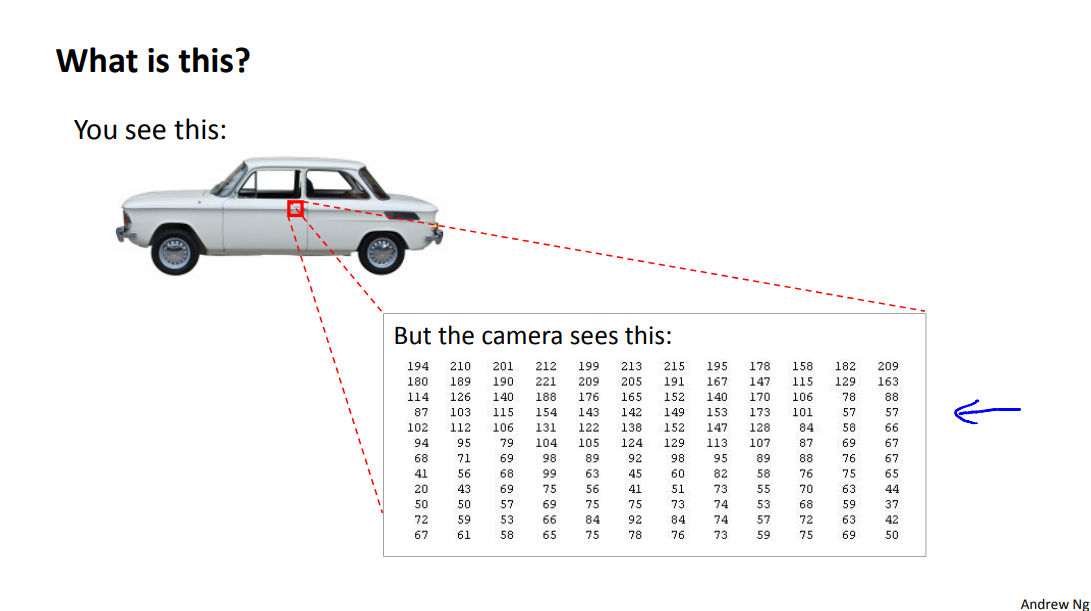
Let's consider the problem of computer vision. And suppose you want to use machine learning to train a classifier to examine an image and tell us whether or not the image is a car. Many people wonder why computer vision could be difficult. I mean when you and I look at this picture it is so obvious what this is. You wonder how is it that a learning algorithm could possibly fail to know what this picture is.

To understand why computer vision is hard let's zoom into a small part of the image like that area where the little red rectangle is. It turns out that where you and I see a car, the computer sees that. What it sees is this matrix, or this grid, of pixel intensity values that tells us the brightness of each pixel in the image. So the computer vision problem is to look at this matrix of pixel intensity values, and tell us that these numbers represent the door handle of a car.

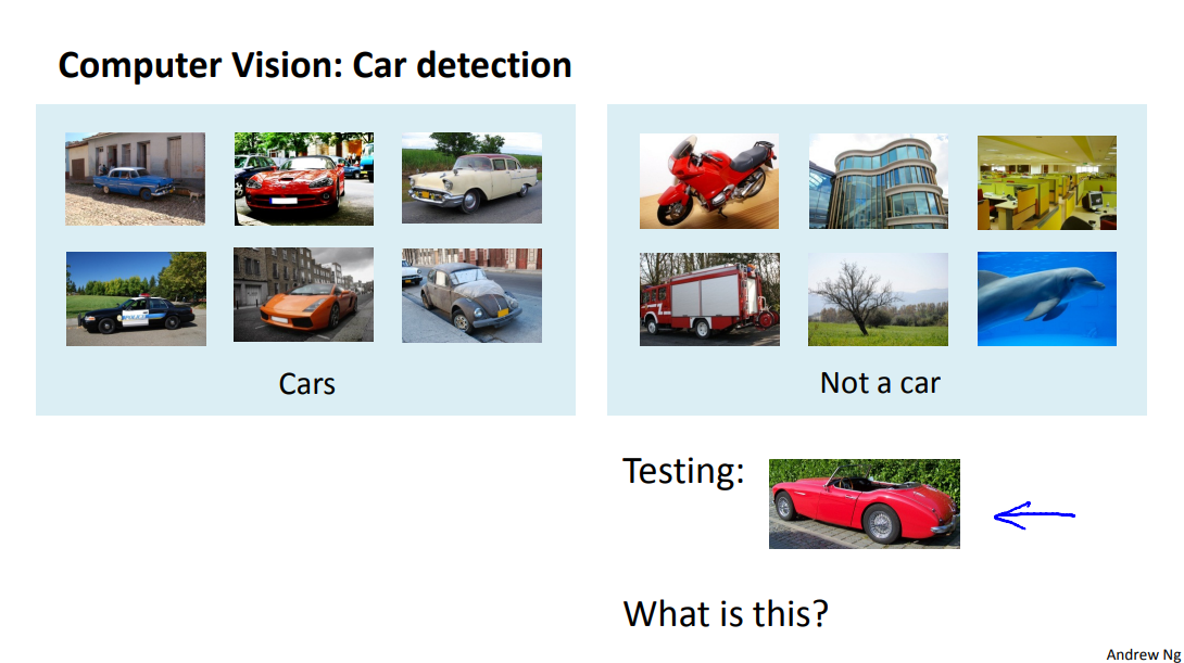
Concretely, when we use machine learning to build a car detector, what we do is we come up with a label training set, with, let's say, a few label examples of cars and a few label examples of things that are not cars, then we give our training set to the learning algorithm trained a classifier and then, you know, we may test it and show the new image and ask, "What is this new thing?". And hopefully it will recognize that that is a car.

To understand why we need nonlinear hypotheses, let's take a look at some of the images of cars and maybe non-cars that we might feed to our learning algorithm.

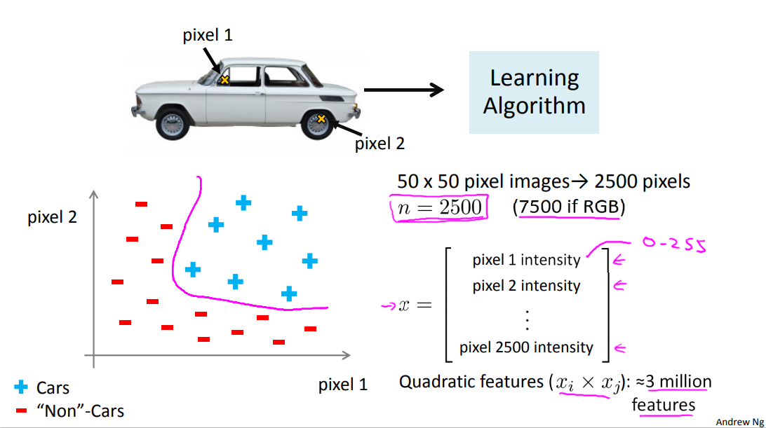
Let's pick a couple of pixel locations in our images, so that's pixel one location and pixel two location, and let's plot this car, you know, at the location, at a certain point, depending on the intensities of pixel one and pixel two.

And let's do this with a few other images. So let's take a different example of the car and you know, look at the same two pixel locations and that image has a different intensity for pixel one and a different intensity for pixel two. So, it ends up at a different location on the figure. And then let's plot some negative examples as well. That's a non-car, that's a non-car . And if we do this for more and more examples using the pluses to denote cars and minuses to denote non-cars, what we'll find is that the cars and non-cars end up lying in different regions of the space, and what we need therefore is some sort of non-linear hypotheses to try to separate out the two classes.

What is the dimension of the feature space? Suppose we were to use just 50 by 50 pixel images. Now that suppose our images were pretty small ones, just 50 pixels on the side. Then we would have 2500 pixels, and so the dimension of our feature size will be N equals 2500 where our feature vector x is a list of all the pixel testings, you know, the pixel brightness of pixel one, the brightness of pixel two, and so on down to the pixel brightness of the last pixel where, you know, in a typical computer representation, each of these may be values between say 0 to 255 if it gives us the grayscale value. So we have n equals 2500, and that's if we were using grayscale images. If we were using RGB images with separate red, green and blue values, we would have n equals 7500.

So, if we were to try to learn a nonlinear hypothesis by including all the quadratic features, that is all the terms of the form, you know, Xi times Xj, while with the 2500 pixels we would end up with a total of three million features. And that's just too large to be reasonable; the computation would be very expensive to find and to represent all of these three million features per training example.

So, simple logistic regression together with adding in maybe the quadratic or the cubic features - that's just not a good way to learn complex nonlinear hypotheses when n is large because you just end up with too many features. In the next few videos, I would like to tell you about Neural Networks, which turns out to be a much better way to learn complex hypotheses, complex nonlinear hypotheses even when your input feature space, even when n is large. And along the way I'll also get to show you a couple of fun videos of historically important applications of Neural networks as well that I hope those videos that we'll see later will be fun for you to watch as well.

1.2 Neurons and the Brain

Neural Networks are a pretty old algorithm that was originally motivated by the goal of having machines that can mimic the brain. Now in this class, of course I'm teaching Neural Networks to you because they work really well for different machine learning problems and not, certainly not because they're logically motivated.

In this video, I'd like to give you some of the background on Neural Networks. So that we can get a sense of what we can expect them to do. Both in the sense of applying them to modern day machinery problems, as well as for those of you that might be interested in maybe the big AI dream of someday building truly intelligent machines. Also, how Neural Networks might pertain to that.

The origins of Neural Networks was as algorithms that try to mimic the brain and those a sense that if we want to build learning systems while why not mimic perhaps the most amazing learning machine we know about, which is perhaps the brain. Neural Networks came to be very widely used throughout the 1980's and 1990's and for various reasons as popularity diminished in the late 90's. But more recently, Neural Networks have had a major recent resurgence.

One of the reasons for this resurgence is that Neural Networks are computationally some what more expensive algorithm and so, it was only, you know, maybe somewhat more recently that computers became fast enough to really run large scale Neural Networks and because of that as well as a few other technical reasons which we'll talk about later, modern Neural Networks today are the state of the art technique for many applications.

So, when you think about mimicking the brain while one of the human brain does tell me same things, right? The brain can learn to see process images than to hear, learn to process our sense of touch. We can, you know, learn to do math, learn to do calculus, and the brain does so many different and amazing things. It seems like if you want to mimic the brain it seems like you have to write lots of different pieces of software to mimic all of these different fascinating, amazing things that the brain tell us, but does is this fascinating hypothesis that the way the brain does all of these different things is not worth like a thousand different programs, but instead, the way the brain does it is worth just a single learning algorithm.

This is just a hypothesis but let me share with you some of the evidence for this. This part of the brain, that little red part of the brain, is your auditory cortex and the way you're understanding my voice now is your ear is taking the sound signal and routing the sound signal to your auditory cortex and that's what's allowing you to understand my words.

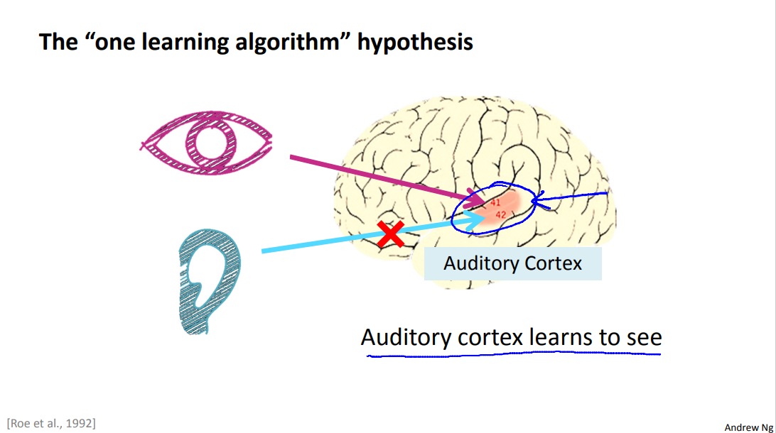
Neuroscientists have done the following fascinating experiments where you cut the wire from the ears to the auditory cortex and you re-wire, in this case an animal's brain, so that the signal from the eyes to the optic nerve eventually gets routed to the auditory cortex. If you do this it turns out, the auditory cortex will learn to see. And this is in every single sense of the word see as we know it. So, if you do this to the animals, the animals can perform visual discrimination task and as they can look at images and make appropriate decisions based on the images and they're doing it with that piece of brain tissue.

Here's another example.

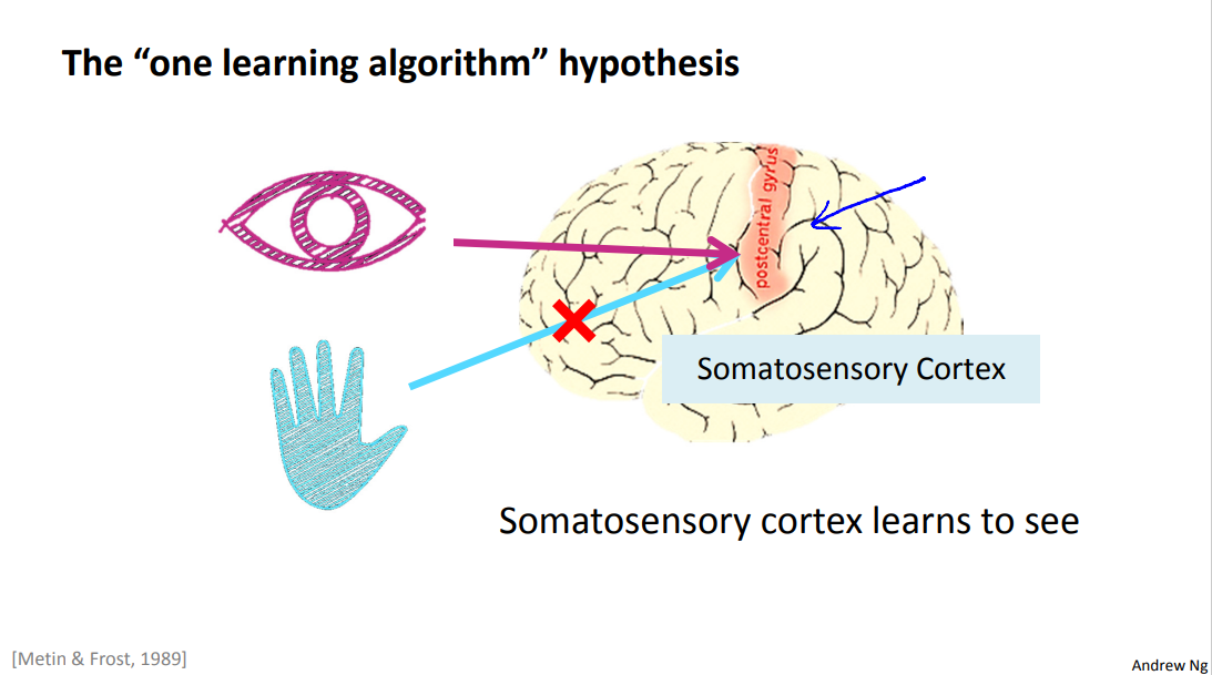
That red piece of brain tissue is your somatosensory cortex. That's how you process your sense of touch. If you do a similar re-wiring process then the somatosensory cortex will learn to see. Because of this and other similar experiments, these are called neuro-rewiring experiments.

There's this sense that if the same piece of physical brain tissue can process sight or sound or touch then maybe there is one learning algorithm that can process sight or sound or touch. And instead of needing to implement a thousand different programs or a thousand different algorithms to do, you know, the thousand wonderful things that the brain does, maybe what we need to do is figure out some approximation or to whatever the brain's learning algorithm is and implement that and that the brain learned by itself how to process these different types of data.

To a surprisingly large extent, it seems as if we can plug in almost any sensor to almost any part of the brain and so, within the reason, the brain will learn to deal with it.

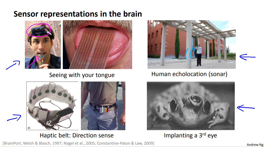
Here are a few more examples. On the upper left is an example of learning to see with your tongue. The way it works is--this is actually a system called BrainPort undergoing FDA trials now to help blind people see--but the way it works is, you strap a grayscale camera to your forehead, facing forward, that takes the low resolution grayscale image of what's in front of you and you then run a wire to an array of electrodes that you place on your tongue so that each pixel gets mapped to a location on your tongue where maybe a high voltage corresponds to a dark pixel and a low voltage corresponds to a bright pixel and, even as it does today, with this sort of system you and I will be able to learn to see, you know, in tens of minutes with our tongues. Here's a second example of human echo location or human sonar.

So there are two ways you can do this. You can either snap your fingers, or click your tongue. I can't do that very well. But there are blind people today that are actually being trained in schools to do this and learn to interpret the pattern of sounds bouncing off your environment - that's sonar. So, if after you search on YouTube, there are actually videos of this amazing kid who tragically because of cancer had his eyeballs removed, so this is a kid with no eyeballs. But by snapping his fingers, he can walk around and never hit anything. He can ride a skateboard. He can shoot a basketball into a hoop and this is a kid with no eyeballs.

Third example is the Haptic Belt where if you have a strap around your waist, ring up buzzers and always have the northmost one buzzing. You can give a human a direction sense similar to maybe how birds can, you know, sense where north is. And, some of the bizarre example, but if you plug a third eye into a frog, the frog will learn to use that eye as well.

So, it's pretty amazing to what extent is as if you can plug in almost any sensor to the brain and the brain's learning algorithm will just figure out how to learn from that data and deal with that data.

And there's a sense that if we can figure out what the brain's learning algorithm is, and, you know, implement it or implement some approximation to that algorithm on a computer, maybe that would be our best shot at, you know, making real progress towards the AI, the artificial intelligence dream of someday building truly intelligent machines.

Now, of course, I'm not teaching Neural Networks, you know, just because they might give us a window into this far-off AI dream, even though I'm personally, that's one of the things that I personally work on in my research life. But the main reason I'm teaching Neural Networks in this class is because it's actually a very effective state of the art technique for modern day machine learning applications.

So, in the next few videos, we'll start diving into the technical details of Neural Networks so that you can apply them to modern-day machine learning applications and get them to work well on problems. But for me, you know, one of the reasons the excite me is that maybe they give us this window into what we might do if we're also thinking of what algorithms might someday be able to learn in a manner similar to humankind.

2 Neural Networks

2.1 Model Representation I

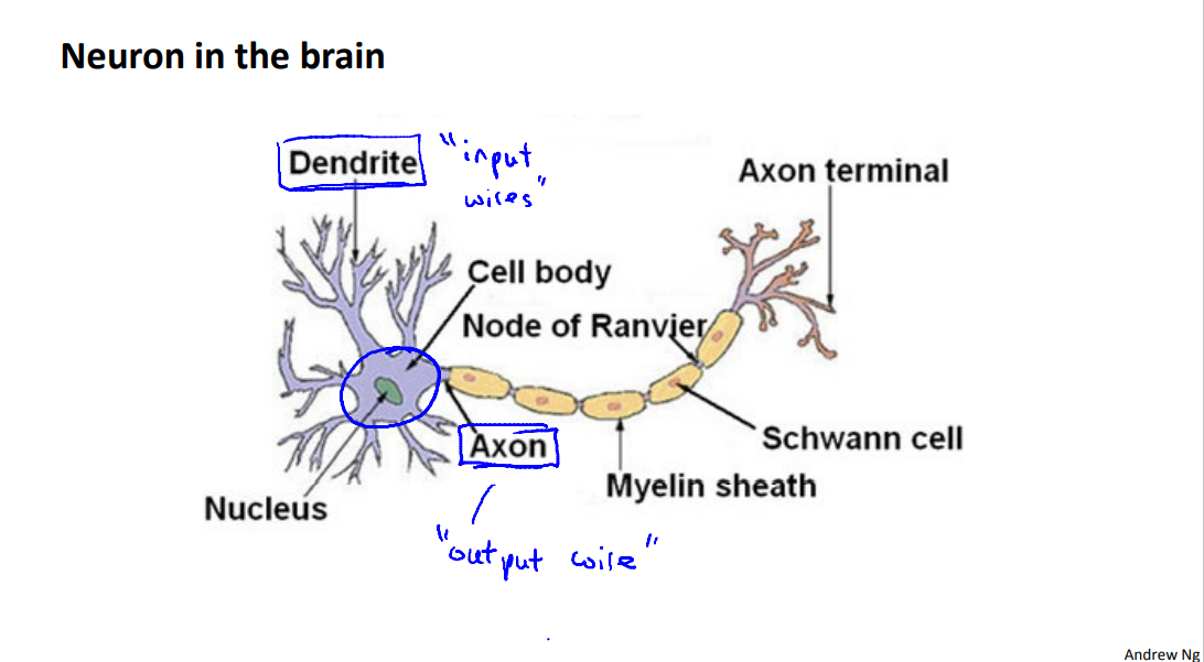
Let's examine how we will represent a hypothesis function using neural networks. Visually, a simplistic representation looks like:

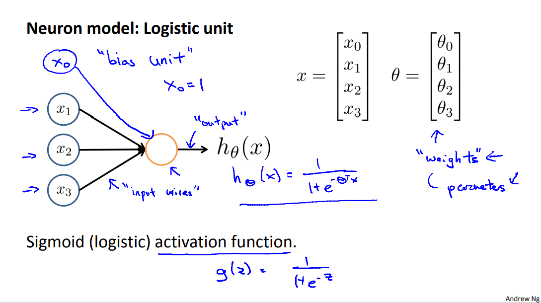
At a very simple level, neurons are basically computational units that take inputs (dendrites) as electrical inputs (called "spikes") that are channeled to outputs (axons). In our model, our dendrites are like the input features $x_1\cdots x_n$ , and the output is the result of our hypothesis function. In this model our $x_0$ input node is sometimes called the "bias unit." It is always equal to 1. In neural networks, we use the same logistic function as in classification, $\frac{1}{1+e^{-{\theta }^{T}x}}$, yet we sometimes call it a sigmoid (logistic) activation function. In this situation, our "theta" parameters are sometimes called "weights".

Our input nodes (layer 1), also known as the "input layer", go into another node (layer 2), which finally outputs the hypothesis function, known as the "output layer".

We can have intermediate layers of nodes between the input and output layers called the "hidden layers."

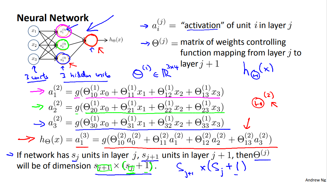
In this example, we label these intermediate or "hidden" layer nodes $a_0^2\cdots a_n^2$ and call them "activation units."

$$\begin{array}{rl}& a_i^{(j)}=\text{"activation" of unit }i\text{ in layer }j\\ & {\mathrm{\Theta }}^{(j)}=\text{matrix of weights controlling function mapping from layer }j\text{ to layer }j+1\end{array}$$

The values for each of the "activation" nodes is obtained as follows:

$$\begin{array}{r}{a}_1^{(2)}=g({\mathrm{\Theta }}_{10}^{(1)}{x}_0+{\mathrm{\Theta }}_{11}^{(1)}{x}_1+{\mathrm{\Theta }}_{12}^{(1)}{x}_2+{\mathrm{\Theta }}_{13}^{(1)}{x}_3)\\ a_2^{(2)}=g({\mathrm{\Theta }}_{20}^{(1)}{x}_0+{\mathrm{\Theta }}_{21}^{(1)}{x}_1+{\mathrm{\Theta }}_{22}^{(1)}{x}_2+{\mathrm{\Theta }}_{23}^{(1)}{x}_3)\\ a_3^{(2)}=g({\mathrm{\Theta }}_{30}^{(1)}{x}_0+{\mathrm{\Theta }}_{31}^{(1)}{x}_1+{\mathrm{\Theta }}_{32}^{(1)}{x}_2+{\mathrm{\Theta }}_{33}^{(1)}{x}_3)\\ h_{\mathrm{\Theta }}(x)=a_1^{(3)}=g({\mathrm{\Theta }}_{10}^{(2)}{a}_0^{(2)}+{\mathrm{\Theta }}_{11}^{(2)}{a}_1^{(2)}+{\mathrm{\Theta }}_{12}^{(2)}{a}_2^{(2)}+{\mathrm{\Theta }}_{13}^{(2)}{a}_3^{(2)})\end{array}$$

This is saying that we compute our activation nodes by using a 3×4 matrix of parameters. We apply each row of the parameters to our inputs to obtain the value for one activation node. Our hypothesis output is the logistic function applied to the sum of the values of our activation nodes, which have been multiplied by yet another parameter matrix ${\mathrm{\Theta }}^{(2)}$ containing the weights for our second layer of nodes.

Each layer gets its own matrix of weights, ${\mathrm{\Theta }}^{(j)}$.

The dimensions of these matrices of weights is determined as follows:

$$\begin{gathered} \text{If network has }{s}_j\text{ units in layer }j\text{ and }{s}_{j+1}\text{ units in layer }j+1\text{, } \\ \text{ then }{\mathrm{\Theta }}^{(j)}\text{ will be of dimension }{s}_{j+1}\times (s_j+1)\text{.} \end{gathered}$$

The +1 comes from the addition in ${\mathrm{\Theta }}^{(j)}$ of the "bias nodes," $x_0$ and ${\mathrm{\Theta }}_0^{(j)}$. In other words the output nodes will not include the bias nodes while the inputs will. The following image summarizes our model representation:

Example: If layer 1 has 2 input nodes and layer 2 has 4 activation nodes. Dimension of ${\mathrm{\Theta }}^{(1)}$ is going to be 4×3 where $s_j=2$ and $s_{j+1}=4$ , so $s_{j+1}\times (s_j+1)=4\times 3$

2.2 Model Representation II

To re-iterate, the following is an example of a neural network:

$$\begin{array}{r}{a}_1^{(2)}=g({\mathrm{\Theta }}_{10}^{(1)}{x}_0+{\mathrm{\Theta }}_{11}^{(1)}{x}_1+{\mathrm{\Theta }}_{12}^{(1)}{x}_2+{\mathrm{\Theta }}_{13}^{(1)}{x}_3)\\ a_2^{(2)}=g({\mathrm{\Theta }}_{20}^{(1)}{x}_0+{\mathrm{\Theta }}_{21}^{(1)}{x}_1+{\mathrm{\Theta }}_{22}^{(1)}{x}_2+{\mathrm{\Theta }}_{23}^{(1)}{x}_3)\\ a_3^{(2)}=g({\mathrm{\Theta }}_{30}^{(1)}{x}_0+{\mathrm{\Theta }}_{31}^{(1)}{x}_1+{\mathrm{\Theta }}_{32}^{(1)}{x}_2+{\mathrm{\Theta }}_{33}^{(1)}{x}_3)\\ h_{\mathrm{\Theta }}(x)=a_1^{(3)}=g({\mathrm{\Theta }}_{10}^{(2)}{a}_0^{(2)}+{\mathrm{\Theta }}_{11}^{(2)}{a}_1^{(2)}+{\mathrm{\Theta }}_{12}^{(2)}{a}_2^{(2)}+{\mathrm{\Theta }}_{13}^{(2)}{a}_3^{(2)})\end{array}$$

In this section we'll do a vectorized implementation of the above functions. We're going to define a new variable $z_k^{(j)}$ that encompasses the parameters inside our g function. In our previous example if we replaced by the variable z for all the parameters we would get:

$$\begin{array}{r}{a}_1^{(2)}=g(z_1^{(2)})\\ a_2^{(2)}=g(z_2^{(2)})\\ a_3^{(2)}=g(z_3^{(2)})\end{array}$$

In other words, for layer j=2 and node k, the variable z will be:

$$z_k^{(2)}={\mathrm{\Theta }}_{k,0}^{(1)}{x}_0+{\mathrm{\Theta }}_{k,1}^{(1)}{x}_1+\cdots +{\mathrm{\Theta }}_{k,n}^{(1)}{x}_n$$

The vector representation of x and $z^j$ is:

$$\begin{array}{rl}x=\left[\begin{array}{c}{x}_0\\ x_1\\ \cdots \\ x_n\end{array}\right]& z^{(j)}=\left[\begin{array}{c}{z}_1^{(j)}\\ z_2^{(j)}\\ \cdots \\ z_n^{(j)}\end{array}\right]\end{array}$$

Setting $x=a^{(1)}$, we can rewrite the equation as:

$$z^{(j)}={\mathrm{\Theta }}^{(j-1)}{a}^{(j-1)}$$

We are multiplying our matrix ${\mathrm{\Theta }}^{(j-1)}$ with dimensions $s_j\times (n+1)$ (where $s_j$ is the number of our activation nodes) by our vector $a^{(j-1)}$ with height (n+1). This gives us our vector $z^{(j)}$ with height $s_j$. Now we can get a vector of our activation nodes for layer j as follows:

$$a^{(j)}=g(z^{(j)})$$

Where our function g can be applied element-wise to our vector $z^{(j)}$

We can then add a bias unit (equal to 1) to layer j after we have computed $a^{(j)}$. This will be element $a_0^{(j)}$ and will be equal to 1. To compute our final hypothesis, let's first compute another z vector:

$$z^{(j+1)}={\mathrm{\Theta }}^{(j)}{a}^{(j)}$$

We get this final z vector by multiplying the next theta matrix after ${\mathrm{\Theta }}^{(j-1)}$ with the values of all the activation nodes we just got. This last theta matrix ${\mathrm{\Theta }}^{(j)}$ will have only one row which is multiplied by one column $a^{(j)}$ so that our result is a single number. We then get our final result with:

$$h_{\mathrm{\Theta }}(x)=a^{(j+1)}=g(z^{(j+1)})$$

Notice that in this last step, between layer j and layer j+1, we are doing exactly the same thing as we did in logistic regression. Adding all these intermediate layers in neural networks allows us to more elegantly produce interesting and more complex non-linear hypotheses.

I'm going to go through a specific example of how a neural network can use this hidden layer there to compute more complex features to feed into this final output layer and how that can learn more complex hypotheses.

3 Applications

3.1 Examples and Intuitions I

A simple example of applying neural networks is by predicting $x_1$ AND $x_2$ , which is the logical 'and' operator and is only true if both $x_1$ and $x_2$ are 1.

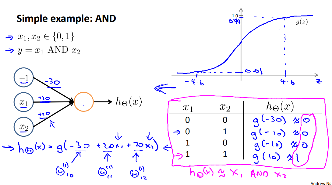
The graph of our functions will look like:

$$\begin{array}{r}\left[\begin{array}{c}{x}_0\\ x_1\\ x_2\end{array}\right]\to \left[\begin{array}{c}g(z^{(2)})\end{array}\right]\to h_{\mathrm{\Theta }}(x)\end{array}$$

Remember that $x_0$ is our bias variable and is always 1.

Let's set our first theta matrix as:

$${\mathrm{\Theta }}^{(1)}=[-302020]$$

his will cause the output of our hypothesis to only be positive if both $x_1$ and $x_2$ are 1. In other words:

$$\begin{array}{rl}& h_{\mathrm{\Theta }}(x)=g(-30+20x_1+20x_2)\\ \\ & x_1=0and{x}_2=0theng(-30)\approx 0\\ & x_1=0and{x}_2=1theng(-10)\approx 0\\ & x_1=1and{x}_2=0theng(-10)\approx 0\\ & x_1=1and{x}_2=1theng(10)\approx 1\end{array}$$

So we have constructed one of the fundamental operations in computers by using a small neural network rather than using an actual AND gate. Neural networks can also be used to simulate all the other logical gates.

The following is an example of the logical operator 'OR', meaning either $x_1$ is true or $x_2$ is true, or both:

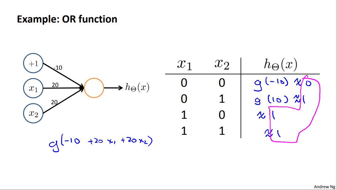
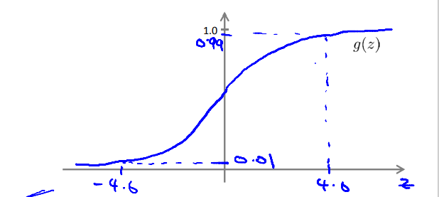
Where g(z) is the following:

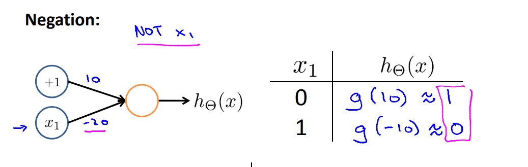
The following is an example of the logical operator 'NOT':

3.2 Examples and Intuitions II

The ${\Theta }^{(1)}$ matrices for AND, NOR, and OR are:

$$\begin{array}{r}AND:\\ {\mathrm{\Theta }}^{(1)}& =\left[\begin{array}{ccc}-30& 20& 20\end{array}\right]\\ NOR:\\ {\mathrm{\Theta }}^{(1)}& =\left[\begin{array}{ccc}10& -20& -20\end{array}\right]\\ OR:\\ {\mathrm{\Theta }}^{(1)}& =\left[\begin{array}{ccc}-10& 20& 20\end{array}\right]\end{array}$$

We can combine these to get the XNOR logical operator (which gives 1 if $x_1$ and $x_2$ are both 0 or both 1).

$$\begin{array}{r}\left[\begin{array}{c}{x}_0\\ x_1\\ x_2\end{array}\right]\to \left[\begin{array}{c}{a}_1^{(2)}\\ a_2^{(2)}\end{array}\right]\to \left[\begin{array}{c}{a}^{(3)}\end{array}\right]\to h_{\mathrm{\Theta }}(x)\end{array}$$

For the transition between the first and second layer, we'll use a ${\Theta }^{(1)}$ matrix that combines the values for AND and NOR:

$${\mathrm{\Theta }}^{(1)}=\left\{\begin{array}{ccc}-30& 10& 20\\ 10& -20& -20\end{array}\right\}$$

For the transition between the second and third layer, we'll use a ${\Theta }^{(2)}$ matrix that uses the value for OR:

$${\mathrm{\Theta }}^{(2)}=[-102020]$$

Let's write out the values for all our nodes:

$$\begin{array}{rl}& a^{(2)}=g({\mathrm{\Theta }}^{(1)}\cdot x)\\ & a^{(3)}=g({\mathrm{\Theta }}^{(2)}\cdot a^{(2)})\\ & h_{\mathrm{\Theta }}(x)=a^{(3)}\end{array}$$

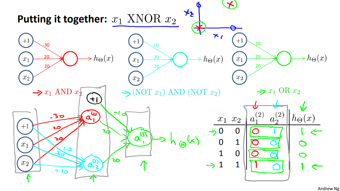
And thus will this neural network, which has a input layer, one hidden layer, and one output layer, we end up with a nonlinear decision boundary that computes this XNOR function. And the more general intuition is that in the input layer, we just have our four inputs. Then we have a hidden layer, which computed some slightly more complex functions of the inputs that its shown here this is slightly more complex functions. And then by adding yet another layer we end up with an even more complex non linear function.

And this is a sort of intuition about why neural networks can compute pretty complicated functions. That when you have multiple layers you have relatively simple function of the inputs of the second layer. But the third layer can build on that to complete even more complex functions, and then the layer after that can compute even more complex functions.

3.3 Multiclass Classification

The way we do multiclass classification in a neural network is essentially an extension of the one versus all method.

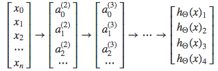
To classify data into multiple classes, we let our hypothesis function return a vector of values. Say we wanted to classify our data into one of four categories. We will use the following example to see how this classification is done. This algorithm takes as input an image and classifies it accordingly:

We can define our set of resulting classes as y:

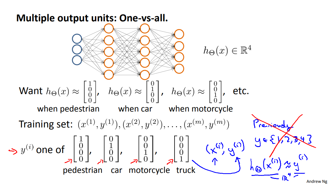
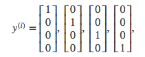
Each $y^{(i)}$ represents a different image corresponding to either a car, pedestrian, truck, or motorcycle. The inner layers, each provide us with some new information which leads to our final hypothesis function. The setup looks like:

Our resulting hypothesis for one set of inputs may look like:

$$h_{\mathrm{\Theta }}(x)=\left[\begin{array}{c}0\\ 0\\ 1\\ 0\end{array}\right]$$

In which case our resulting class is the third one down, or $h_{\mathrm{\Theta }}(x{)}_3$, which represents the motorcycle.