Machine Learning Week_3 Classification Model

目录

• 1 Classification and Representation
  • 1.1 Classification
    • unfamiliar words
  • 1.2 Hypothesis Representation
    • unfamiliar words
  • 1.3 Decision Boundary
• 2 Logistic Regeression Model
  • 2.1 Cost Function
    • unfamiliar words
  • 2.2 Simplified Cost Function and Gradient Descent
  • 2.3 Advanced Optimization
    • unfamiliar words
• 3 Multiclass Classification
  • 3.1 Multiclass Classification: One-vs-all
• 4 Solving The Problem of Overfitting
  • 4.1 The Problem of Overfitting
    • unfamiliar words
  • 4.2 Cost Function
    • unfamiliar words
  • 4.3 Regularized Linear Regression
  • 4.4 Regularized Logistic Regression

1 Classification and Representation

1.1 Classification

• Emali: Spam | Not Spam
• Tumot: Malignant | Benign
• Online Transcations: Fraudulent (Yes | NO)

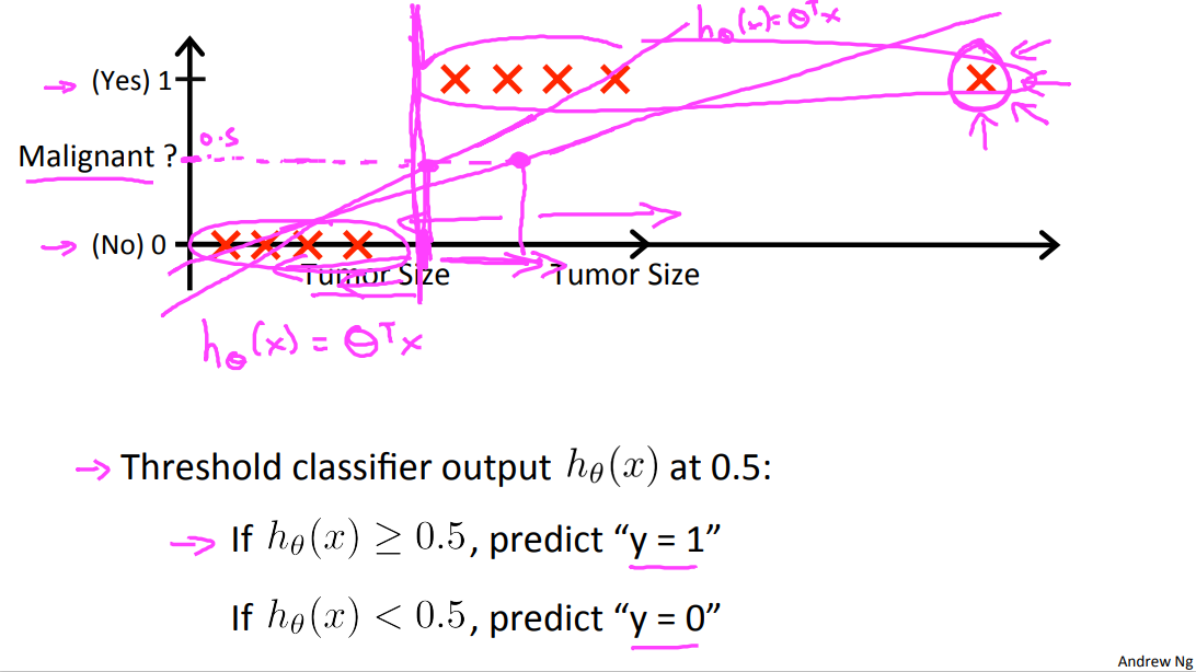
So how do we develop a classification algorithm? Here's an example of a training set for a classification task for classifying a tumor as malignant or benign. And notice that malignancy takes on only two values, zero or no, one or yes. So one thing we could do given this training set is to apply the algorithm that we already know.

Linear regression to this data set and just try to fit the straight line to the data. So if you take this training set and fill a straight line to it, maybe you get a hypothesis that looks like that, right. So that's my hypothesis. H(x) equals theta transpose x. If you want to make predictions one thing you could try doing is then threshold the classifier outputs at 0.5 that is at a vertical axis value 0.5 and if the hypothesis outputs a value that is greater than equal to 0.5 you can take y = 1. If it's less than 0.5 you can take y=0. Let's see what happens if we do that. So 0.5 and so that's where the threshold is and that's using linear regression this way. Everything to the right of this point we will end up predicting as the positive cross. Because the output values is greater than 0.5 on the vertical axis and everything to the left of that point we will end up predicting as a negative value.

In this particular example, it looks like linear regression is actually doing something reasonable. Even though this is a classification task we're interested in. But now let's try changing the problem a bit. Let me extend out the horizontal access a little bit and let's say we got one more training example way out there on the right. Notice that that additional training example, this one out here, it doesn't actually change anything, right. Looking at the training set it's pretty clear what a good hypothesis is. Is that well everything to the right of somewhere around here, to the right of this we should predict this positive. Everything to the left we should probably predict as negative because from this training set, it looks like all the tumors larger than a certain value around here are malignant, and all the tumors smaller than that are not malignant, at least for this training set.

But once we've added that extra example over here, if you now run linear regression, you instead get a straight line fit to the data. That might maybe look like this.And if you know threshold hypothesis at 0.5, you end up with a threshold that's around here, so that everything to the right of this point you predict as positive and everything to the left of that point you predict as negative.And this seems a pretty bad thing for linear regression to have done, right, because you know these are our positive examples, these are our negative examples. It's pretty clear we really should be separating the two somewhere around there, but somehow by adding one example way out here to the right, this example really isn't giving us any new information. I mean, there should be no surprise to the learning algorithm. That the example way out here turns out to be malignant. But somehow having that example out there caused linear regression to change its straight-line fit to the data from this magenta line out here to this blue line over here, and caused it to give us a worse hypothesis.

So, applying linear regression to a classification problem often isn't a great idea. In the first example, before I added this extra training example, previously linear regression was just getting lucky and it got us a hypothesis that worked well for that particular example, but usually applying linear regression to a data set, you might get lucky but often it isn't a good idea.So I wouldn't use linear regression for classification problems.

To attempt classification, one method is to use linear regression and map all predictions greater than 0.5 as a 1 and all less than 0.5 as a 0. However, this method doesn't work well because classification is not actually a linear function.

The classification problem is just like the regression problem, except that the values we now want to predict take on only a small number of discrete values. For now, we will focus on the binary classification problem in which y can take on only two values, 0 and 1. (Most of what we say here will also generalize to the multiple-class case.) For instance, if we are trying to build a spam classifier for email, then $x^{(i)}$ may be some features of a piece of email, and y may be 1 if it is a piece of spam mail, and 0 otherwise. Hence, y∈{0,1}. 0 is also called the negative class, and 1 the positive class, and they are sometimes also denoted by the symbols “-” and “+.” Given $x^{(i)}$, the corresponding $y^{(i)}$ is also called the label for the training example.

Here's one other funny thing about what would happen if we were to use linear regression for a classification problem. For classification we know that y is either zero or one. But if you are using linear regression where the hypothesis can output values that are much larger than one or less than zero, even if all of your training examples have labels y equals zero or one.

So what we'll do in the next few videos is develop an algorithm called logistic regression, which has the property that the output, the predictions of logistic regression are always between zero and one, and doesn't become bigger than one or become less than zero.

And by the way, logistic regression is, and we will use it as a classification algorithm, is some, maybe sometimes confusing that the term regression appears in this name even though logistic regression is actually a classification algorithm. But that's just a name it was given for historical reasons. So don't be confused by that logistic regression is actually a classification algorithm that we apply to settings where the label y is discrete value, when it's either zero or one. So hopefully you now know why, if you have a classification problem, using linear regression isn't a good idea. In the next video, we'll start working out the details of the logistic regression algorithm.

unfamiliar words

1. Fraudulent [ˈfrɔːdjʊlənt] adj.欺骗的；欺诈的
   The scheme seems to be much better than fraudulent public works of the past, having officially provided work to over 47m households.
   这项计划已使四千七百多万居民受惠，似乎比从前那些欺骗民众的工作要强的多。

1.2 Hypothesis Representation

We could approach the classification problem ignoring the fact that y is discrete-valued, and use our old linear regression algorithm to try to predict y given x. However, it is easy to construct examples where this method performs very poorly. Intuitively, it also doesn’t make sense for $h_{\theta }(x)$ to take values larger than 1 or smaller than 0 when we know that y ∈ {0, 1}. To fix this, let’s change the form for our hypotheses $h_{\theta }(x)$ to satisfy $0\le h_{\theta }(x)\le 1$. This is accomplished by plugging ${\theta }^{T}x$ into the Logistic Function.

Our new form uses the "Sigmoid Function," also called the "Logistic Function":

$$\begin{array}{rl}& h_{\theta }(x)=g({\theta }^{T}x)\\ \\ & z={\theta }^{T}x\\ & g(z)={\displaystyle \frac{1}{1+e^{-z}}}\end{array}$$

The following image shows us what the sigmoid function looks like:

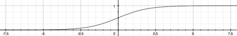
The function g(z), shown here, maps any real number to the (0, 1) interval, making it useful for transforming an arbitrary-valued function into a function better suited for classification.

$h_{\theta }(x)$ will give us the probability that our output is 1. For example, $h_{\theta }(x)=0.7$ gives us a probability of 70% that our output is 1. Our probability that our prediction is 0 is just the complement of our probability that it is 1 (e.g. if probability that it is 1 is 70%, then the probability that it is 0 is 30%).

$$\begin{array}{rl}& h_{\theta }(x)=P(y=1|x;\theta )=1-P(y=0|x;\theta )\\ & P(y=0|x;\theta )+P(y=1|x;\theta )=1\end{array}$$

Just like $P(A|B)$.

unfamiliar words

1. complement [ˈkɑmpləˌment] v.补充；补足；使完美；使更具吸引力 n.补语；补足语；补充物；补足物
   V. The excellent menu is complemented by a good wine list. 佳肴佐以美酒，可称完美无缺。
   N. But I knew Dick would be a strong complement to me, and this has proven to be the case. 但是我知道，Dick将会是我的得力助手，事实证明确实如此。

1.3 Decision Boundary

In order to get our discrete 0 or 1 classification, we can translate the output of the hypothesis function as follows:

$$\begin{array}{rl}& h_{\theta }(x)\ge 0.5\to y=1\\ & h_{\theta }(x)<0.5\to y=0\end{array}$$

The way our logistic function g behaves is that when its input is greater than or equal to zero, its output is greater than or equal to 0.5:

$$\begin{array}{rl}& g(z)\ge 0.5\\ & whenz\ge 0\end{array}$$

Remember.

$$\begin{array}{r}z=0,e^0=1\Rightarrow g(z)=1/2\\ z\to \mathrm{\infty },e^{-\mathrm{\infty }}\to 0\Rightarrow g(z)=1\\ z\to -\mathrm{\infty },e^{\mathrm{\infty }}\to \mathrm{\infty }\Rightarrow g(z)=0\end{array}$$

So if our input to g is ${\theta }^{T}X$, then that means:

$$\begin{array}{rl}& h_{\theta }(x)=g({\theta }^{T}x)\ge 0.5\\ & when{\theta }^{T}x\ge 0\end{array}$$

From these statements we can now say:

$$\begin{array}{rl}& {\theta }^{T}x\ge 0\Rightarrow y=1\\ & {\theta }^{T}x<0\Rightarrow y=0\end{array}$$

The decision boundary is the line that separates the area where y = 0 and where y = 1. It is created by our hypothesis function.

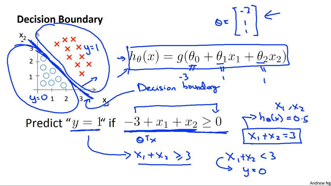
Using the formulas that we were taught on the previous slide, we know that y equals one is more likely, that is the probability that y equals one is greater than or equal to 0.5, whenever theta transpose x is greater than zero. And this formula that I just underlined, -3 + x1 + x2, is, of course, theta transpose x when theta is equal to this value of the parameters that we just chose.

So for any example, for any example which features x1 and x2 that satisfy this equation, that minus 3 plus x1 plus x2 is greater than or equal to 0, our hypothesis will think that y equals 1, the small x will predict that y is equal to 1.

We can also take -3 and bring this to the right and rewrite this as x1+x2 is greater than or equal to 3, so equivalently, we found that this hypothesis would predict y=1 whenever x1+x2 is greater than or equal to 3.

Let's see what that means on the figure, if I write down the equation, X1 + X2 = 3, this defines the equation of a straight line and if I draw what that straight line looks like, it gives me the following line which passes through 3 and 3 on the x1 and the x2 axis.

So the part of the infospace, the part of the X1 X2 plane that corresponds to when X1 plus X2 is greater than or equal to 3, that's going to be this right half thing, that is everything to the up and everything to the upper right portion of this magenta line that I just drew. And so, the region where our hypothesis will predict y = 1, is this region, just really this huge region, this half space over to the upper right. And let me just write that down, I'm gonna call this the y = 1 region. And, in contrast, the region where x1 + x2 is less than 3, that's when we will predict that y is equal to 0. And that corresponds to this region. And there's really a half plane, but that region on the left is the region where our hypothesis will predict y = 0. I wanna give this line, this magenta line that I drew a name. This line, there, is called the decision boundary.

And concretely, this straight line, X1 plus X equals 3. That corresponds to the set of points, so that corresponds to the region where H of X is equal to 0.5 exactly and the decision boundary that is this straight line, that's the line that separates the region where the hypothesis predicts Y equals 1 from the region where the hypothesis predicts that y is equal to zero. And just to be clear, the decision boundary is a property of the hypothesis including the parameters theta zero, theta one, theta two. And in the figure I drew a training set, I drew a data set, in order to help the visualization. But even if we take away the data set this decision boundary and the region where we predict y =1 versus y = 0, that's a property of the hypothesis and of the parameters of the hypothesis and not a property of the data set.

Example:

$$\begin{array}{rl}& \theta =\left[\begin{array}{c}5\\ -1\\ 0\end{array}\right]\\ & y=1if5+(-1)x_1+0x_2\ge 0\\ & 5-x_1\ge 0\\ & -x_1\ge -5\\ & x_1\le 5\end{array}$$

In this case, our decision boundary is a straight vertical line placed on the graph where $x_1=5$, and everything to the left of that denotes y = 1, while everything to the right denotes y = 0.

None-Linear decision boundaries

Earlier when we were talking about polynomial regression or when we're talking about linear regression, we talked about how we could add extra higher order polynomial terms to the features. And we can do the same for logistic regression. Concretely, let's say my hypothesis looks like this where I've added two extra features, x1 squared and x2 squared, to my features. So that I now have five parameters, theta zero through theta four.

As before, we'll defer to the next video, our discussion on how to automatically choose values for the parameters theta zero through theta four. But let's say that varied procedure to be specified, I end up choosing theta zero equals minus one, theta one equals zero, theta two equals zero, theta three equals one and theta four equals one.

What this means is that with this particular choose of parameters, my parameter effect theta theta looks like minus one, zero, zero, one, one.

Following our earlier discussion, this means that my hypothesis will predict that y=1 whenever -1 + x1 squared + x2 squared is greater than or equal to 0. This is whenever theta transpose times my theta transfers, my features is greater than or equal to zero. And if I take minus 1 and just bring this to the right, I'm saying that my hypothesis will predict that y is equal to 1 whenever x1 squared plus x2 squared is greater than or equal to 1. So what does this decision boundary look like? Well, if you were to plot the curve for x1 squared plus x2 squared equals 1 Some of you will recognize that, that is the equation for circle of radius one, centered around the origin. So that is my decision boundary.

And everything outside the circle, I'm going to predict as y=1. So out here is my y equals 1 region, we'll predict y equals 1 out here and inside the circle is where I'll predict y is equal to 0. So by adding these more complex, or these polynomial terms to my features as well, I can get more complex decision boundaries that don't just try to separate the positive and negative examples in a straight line that I can get in this example, a decision boundary that's a circle.

Once again, the decision boundary is a property, not of the trading set, but of the hypothesis under the parameters. So, so long as we're given my parameter vector theta, that defines the decision boundary, which is the circle. But the training set is not what we use to define the decision boundary. The training set may be used to fit the parameters theta. We'll talk about how to do that later. But, once you have the parameters theta, that is what defines the decisions boundary.

Again, the input to the sigmoid function g(z) (e.g. ${\theta }^{T}X$ doesn't need to be linear, and could be a function that describes a circle (e.g. $z={\theta }_0+{\theta }_1{x}_1^2+{\theta }_2{x}_2^2$ ) or any shape to fit our data.

2 Logistic Regeression Model

2.1 Cost Function

We cannot use the same cost function that we use for linear regression because the Logistic Function(or Sigmoid Function) will cause the output to be wavy, causing many local optima. In other words, it will not be a convex function.

Instead, our cost function for logistic regression looks like:

$$\begin{array}{rl}& J(\theta )={\displaystyle \frac{1}{m}}\sum _{i=1}^m\mathrm{Cost}(h_{\theta }(x^{(i)}),y^{(i)})\\ & \mathrm{Cost}(h_{\theta }(x),y)=-\log (h_{\theta }(x))& \text{if y = 1}\\ & \mathrm{Cost}(h_{\theta }(x),y)=-\log (1-h_{\theta }(x))& \text{if y = 0}\end{array}$$

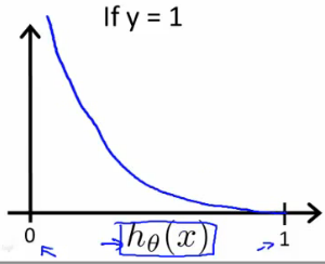
When y = 1, we get the following plot for $J(\theta )$ vs $h_{\theta }(x)$ :

Similarly, when y = 0, we get the following plot for $J(\theta )$ vs $h_{\theta }(x)$ :

$$\begin{array}{rl}& \mathrm{Cost}(h_{\theta }(x),y)=0\text{ if }{h}_{\theta }(x)=y\\ & \mathrm{Cost}(h_{\theta }(x),y)\to \mathrm{\infty }\text{ if }y=0\mathrm{and}{h}_{\theta }(x)\to 1\\ & \mathrm{Cost}(h_{\theta }(x),y)\to \mathrm{\infty }\text{ if }y=1\mathrm{and}{h}_{\theta }(x)\to 0\end{array}$$

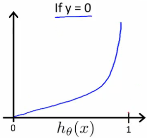
If our correct answer 'y' is 0, then the cost function will be 0 if our hypothesis function also outputs 0. If our hypothesis approaches 1, then the cost function will approach infinity.

If our correct answer 'y' is 1, then the cost function will be 0 if our hypothesis function outputs 1. If our hypothesis approaches 0, then the cost function will approach infinity.

Note that writing the cost function in this way guarantees that J(θ) is convex for logistic regression.

The topic of convexity analysis is now beyond the scope of this course, but it is possible to show that with a particular choice of cost function, this will give a convex optimization problem. Overall cost function j of theta will be convex and local optima free.

unfamiliar words

1. wavy [ˈweɪvi] adj. 起伏不平的;波浪形的;拳曲的
   She had short, wavy brown hair.
   她留着微卷的褐色短发。

2. penalty [ˈpenəlti] n. 处罚;刑罚;惩罚;害处;不利;(对犯规者的)判罚
   exp: N a punishment for breaking a law, rule or contract
   to impose a penalty
   予以惩罚
   We are goingto say the cost or the penalty that the algorithem pays.

2.2 Simplified Cost Function and Gradient Descent

Note: [6:53 - the gradient descent equation should have a 1/m factor]

And just want to remind you that for classification problems in our training sets, and in fact even for examples, now that our training set y is always equal to zero or one, right? That's sort of part of the mathematical definition of y.

**Because y is either zero or one, we'll be able to come up with a simpler way to write this cost function. **

We can compress our cost function's two conditional cases into one case:

$$\mathrm{Cost}(h_{\theta }(x),y)=-y\log (h_{\theta }(x))-(1-y)\log (1-h_{\theta }(x))$$

Notice that when y is equal to 1, then the second term $(1-y)\log (1-h_{\theta }(x))$ will be zero and will not affect the result. If y is equal to 0, then the first term $-y\log (h_{\theta }(x))$ will be zero and will not affect the result.

We can fully write out our entire cost function as follows:

$$J(\theta )=-\frac{1}{m}{\displaystyle \sum _{i=1}^m[y^{(i)}\log (h_{\theta }(x^{(i)}))+(1-y^{(i)})\log (1-h_{\theta }(x^{(i)}))]}$$

Although I won't have time to go into great detail of this in this course, this cost function can be derived from statistics using the principle of maximum likelihood estimation. Which is an idea in statistics for how to efficiently find parameters' data for different models. And it also has a nice property that it is convex. So this is the cost function that essentially everyone uses when fitting logistic regression models. If you don't understand the terms that I just said, if you don't know what the principle of maximum likelihood estimation is, don't worry about it. But it's just a deeper rationale and justification behind this particular cost function than I have time to go into in this class.

A vectorized implementation is:

$$\begin{array}{rl}& h=g(X\theta )\\ & J(\theta )=\frac{1}{m}\cdot (-y^T\log (h)-(1-y{)}^T\log (1-h))\end{array}$$

Gradient Descent

Remember that the general form of gradient descent is:

$$\begin{array}{rl}& Repeat\{\\ & {\theta }_j:={\theta }_j-\alpha {\displaystyle \frac{\partial }{\partial {\theta }_j}}J(\theta )\\ & \}\end{array}$$

We can work out the derivative part using calculus to get:

$$\begin{array}{rl}& Repeat\{\\ & {\theta }_j:={\theta }_j-\frac{\alpha }{m}\sum _{i=1}^m(h_{\theta }(x^{(i)})-y^{(i)})x_j^{(i)}\\ & \}\end{array}$$

Now, if you take this update rule and compare it to what we were doing for linear regression. You might be surprised to realize that, well, this equation($h_{\theta }(x)=g({\theta }^{T}X$) was exactly what we had for linear regression($h_{\theta }(x)={\theta }^{T}X$). So even though the update rule looks cosmetically identical, because the definition of the hypothesis has changed, this is actually not the same thing as gradient descent for linear regression.

Notice that this algorithm is identical to the one we used in linear regression. We still have to simultaneously update all values in theta.

A vectorized implementation is:

$$\theta :=\theta -\frac{\alpha }{m}{X}^T(g(X\theta )-\overrightarrow{y})$$

In an earlier video, when we were talking about gradient descent for linear regression, we had talked about how to monitor a gradient descent to make sure that it is converging. I usually apply that same method to logistic regression, too to monitor a gradient descent, to make sure it's converging correctly. And hopefully, you can figure out how to apply that technique to logistic regression yourself.

2.3 Advanced Optimization

Note: [7:35 - '100' should be 100 instead. The value provided should be an integer and not a character string.]

In this video, I'd like to tell you about some advanced optimization algorithms and some advanced optimization concepts. Using some of these ideas, we'll be able to get logistic regression to run much more quickly than it's possible with gradient descent. And this will also let the algorithms scale much better to very large machine learning problems, such as if we had a very large number of features.

So, having written code to compute these two things, one algorithm we can use is gradient descent.

$$\begin{array}{rl}& J(\theta )\\ & {\displaystyle \frac{\partial }{\partial {\theta }_j}}J(\theta )\end{array}$$

But gradient descent isn't the only algorithm we can use. And there are other algorithms, more advanced, more sophisticated ones, that, if we only provide them a way to compute these two things, then these are different approaches to optimize the cost function for us.

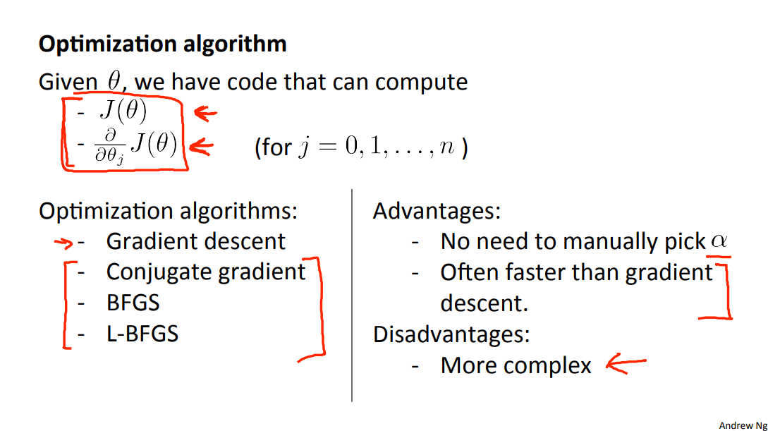
So conjugate gradient BFGS and L-BFGS are examples of more sophisticated optimization algorithms that need a way to compute J of theta, and need a way to compute the derivatives, and can then use more sophisticated strategies than gradient descent to minimize the cost function.The details of exactly what these three algorithms is well beyond the scope of this course. And in fact you often end up spending, you know, many days, or a small number of weeks studying these algorithms. If you take a class and advance the numerical computing.

But let me just tell you about some of their properties.These three algorithms have a number of advantages. One is that, with any of this algorithms you usually do not need to manually pick the learning rate alpha.So one way to think of these algorithms is that given is the way to compute the derivative and a cost function. You can think of these algorithms as having a clever inter-loop. And, in fact, they have a clever inter-loop called a line search algorithm that automatically tries out different values for the learning rate alpha and automatically picks a good learning rate alpha so that it can even pick a different learning rate for every iteration. And so then you don't need to choose it yourself.

These algorithms actually do more sophisticated things than just pick a good learning rate, and so they often end up converging much faster than gradient descent.

These algorithms actually do more sophisticated things than just pick a good learning rate, and so they often end up converging much faster than gradient descent, but detailed discussion of exactly what they do is beyond the scope of this course.

In fact, I actually used to have used these algorithms for a long time, like maybe over a decade, quite frequently, and it was only, you know, a few years ago that I actually figured out for myself the details of what conjugate gradient, BFGS and O-BFGS do. So it is actually entirely possible to use these algorithms successfully and apply to lots of different learning problems without actually understanding the inter-loop of what these algorithms do.

If these algorithms have a disadvantage, I'd say that the main disadvantage is that they're quite a lot more complex than gradient descent. And in particular, you probably should not implement these algorithms - conjugate gradient, L-BGFS, BFGS - yourself unless you're an expert in numerical computing.

Instead, just as I wouldn't recommend that you write your own code to compute square roots of numbers or to compute inverses of matrices, for these algorithms also what I would recommend you do is just use a software library. So, you know, to take a square root what all of us do is use some function that someone else has written to compute the square roots of our numbers.

And fortunately, Octave and the closely related language MATLAB - we'll be using that - Octave has a very good. Has a pretty reasonable library implementing some of these advanced optimization algorithms. And so if you just use the built-in library, you know, you get pretty good results.

I should say that there is a difference between good and bad implementations of these algorithms. And so, if you're using a different language for your machine learning application, if you're using C, C++, Java, and so on, you might want to try out a couple of different libraries to make sure that you find a good library for implementing these algorithms. Because there is a difference in performance between a good implementation of, you know, contour gradient or LPFGS versus less good implementation of contour gradient or LPFGS.

"Conjugate gradient", "BFGS", and "L-BFGS" are more sophisticated, faster ways to optimize θ that can be used instead of gradient descent. We suggest that you should not write these more sophisticated algorithms yourself (unless you are an expert in numerical computing) but use the libraries instead, as they're already tested and highly optimized. Octave provides them.

We first need to provide a function that evaluates the following two functions for a given input value θ:

$$\begin{array}{rl}& J(\theta )\\ & {\displaystyle \frac{\partial }{\partial {\theta }_j}}J(\theta )\end{array}$$

We can write a single function that returns both of these:

function [jVal, gradient] = costFunction(theta)
  jVal = [...code to compute J(theta)...];
  gradient = [...code to compute derivative of J(theta)...];
end

Then we can use octave's "fminunc()" optimization algorithm along with the "optimset()" function that creates an object containing the options we want to send to "fminunc()". (Note: the value for MaxIter should be an integer, not a character string - errata in the video at 7:30)

options = optimset('GradObj', 'on', 'MaxIter', 100);
initialTheta = zeros(2,1);
   [optTheta, functionVal, exitFlag] = fminunc(@costFunction, initialTheta, options);

We give to the function "fminunc()" our cost function, our initial vector of theta values, and the "options" object that we created beforehand.

So, now you know how to use these advanced optimization algorithms. Because, using, because for these algorithms, you're using a sophisticated optimization library, it makes the just a little bit more opaque and so just maybe a little bit harder to debug. But because these algorithms often run much faster than gradient descent, often quite typically whenever I have a large machine learning problem, I will use these algorithms instead of using gradient descent.

And with these ideas, hopefully, you'll be able to get logistic progression and also linear regression to work on much larger problems. So, that's it for advanced optimization concepts.

unfamiliar words

1. sophisticated 英 [səˈfɪstɪkeɪtɪd] adj. 复杂的;精密的;先进的;
   • exp1：ADJ having a lot of experience of the world and knowing about fashion, culture and other things that people think are socially important 见多识广的；老练的；
     Mark is a smart and sophisticated young man.
     马克是一个聪明老成的年轻人。
   • clever and complicated in the way that it works or is presented 先进的；精密的
     highly sophisticated computer systems
     十分先进的计算机系统

3 Multiclass Classification

3.1 Multiclass Classification: One-vs-all

• Email folder/tagging: Work, Friends, Family, Hobby.
• Medical diagrams: Not ill, Cold, Flu.
• Weather: Sunny, Cloudy, Rain, Snow.u

Now we will approach the classification of data when we have more than two categories. Instead of y = {0,1} we will expand our definition so that y = {0,1...n}.

Since y = {0,1...n}, we divide our problem into n+1 (+1 because the index starts at 0) binary classification problems; in each one, we predict the probability that 'y' is a member of one of our classes.

$$\begin{array}{rl}& y\in \{0,1...n\}\\ & h_{\theta }^{(0)}(x)=P(y=0|x;\theta )\\ & h_{\theta }^{(1)}(x)=P(y=1|x;\theta )\\ & \cdots \\ & h_{\theta }^{(n)}(x)=P(y=n|x;\theta )\\ & \mathrm{prediction}=\underset{i}{max}(h_{\theta }^{(i)}(x))\end{array}$$

We are basically choosing one class and then lumping all the others into a single second class. We do this repeatedly, applying binary logistic regression to each case, and then use the hypothesis that returned the highest value as our prediction.

The following image shows how one could classify 3 classes:

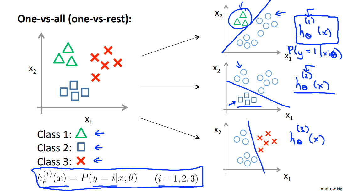
Here's how a one-vs-all classification works. And this is also sometimes called one-vs-rest. Let's say we have a training set like that shown on the left, where we have three classes of y equals 1, we denote that with a triangle, if y equals 2, the square, and if y equals three, then the cross.

What we're going to do is take our training set and turn this into three separate binary classification problems. I'll turn this into three separate two class classification problems. So let's start with class one which is the triangle. We're gonna essentially create a new sort of fake training set where classes two and three get assigned to the negative class. And class one gets assigned to the positive class. You want to create a new training set like that shown on the right, and we're going to fit a classifier which I'm going to call h subscript theta superscript one of x where here the triangles are the positive examples and the circles(the rest of the class1) are the negative examples.

So think of the triangles being assigned the value of one and the circles assigned the value of zero. And we're just going to train a standard logistic regression classifier and maybe that will give us a position boundary that looks like that.

To summarize:

Train a logistic regression classifier $h_{\theta }^{(i)}(x)$ for each class $i$ to predict the probability that $y=i$.

To make a prediction on a new x, pick the class that maximizes $h_{\theta }^{(i)}(x)$.

4 Solving The Problem of Overfitting

4.1 The Problem of Overfitting

Consider the problem of predicting y from x ∈ R. The leftmost figure below shows the result of fitting a $y={\theta }_0+{\theta }_{1}x$ to a dataset. We see that the data doesn’t really lie on straight line, and so the fit is not very good.

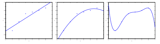
Instead, if we had added an extra feature $x^2$, and fit $y={\theta }_0+{\theta }_{1}x+{\theta }_2{x}^2$, then we obtain a slightly better fit to the data (See middle figure). Naively, it might seem that the more features we add, the better. However, there is also a danger in adding too many features: The rightmost figure is the result of fitting a $5^{th}$ order polynomial $y=\sum _{j=0}^5{\theta }_j{x}^j$. We see that even though the fitted curve passes through the data perfectly, we would not expect this to be a very good predictor of, say, housing prices (y) for different living areas (x). Without formally defining what these terms mean, we’ll say the figure on the left shows an instance of underfitting—in which the data clearly shows structure not captured by the model—and the figure on the right is an example of overfitting.

Underfitting, or high bias, is when the form of our hypothesis function h maps poorly to the trend of the data. It is usually caused by a function that is too simple or uses too few features. At the other extreme, overfitting, or high variance, is caused by a hypothesis function that fits the available data but does not generalize well to predict new data. It is usually caused by a complicated function that creates a lot of unnecessary curves and angles unrelated to the data.

This terminology is applied to both linear and logistic regression. There are two main options to address the issue of overfitting:

1 Reduce the number of features:

• Manually select which features to keep.

• Use a model selection algorithm (studied later in the course).

2 Regularization

• Keep all the features, but reduce the magnitude of parameters ${\theta }_j$.

• Regularization works well when we have a lot of slightly useful features.

unfamiliar words

1. naively [nɑˈi:vlɪ] adv. 无邪地；天真烂漫地
   Many seem to naively believe that we won't run out of the resources we need to keep this system going.
   许多人天真地认为，我们不会耗尽所有的资源，我们必须让这个系统持续运转下去。

4.2 Cost Function

Note: [5:18 - There is a typo. It should be $\sum _{j=1}^n{\theta }_j^2$ instead of $\sum _{i=1}^n{\theta }_j^2$]

If we have overfitting from our hypothesis function, we can reduce the weight that some of the terms in our function carry by increasing their cost.

Say we wanted to make the following function more quadratic:

$${\theta }_0+{\theta }_{1}x+{\theta }_2{x}^2+{\theta }_3{x}^3+{\theta }_4{x}^4$$

We'll want to eliminate the influence of ${\theta }_3{x}^3$ and ${\theta }_4{x}^4$. Without actually getting rid of these features or changing the form of our hypothesis, we can instead modify our cost function:

$$mi{n}_{\theta }{\displaystyle \frac{1}{2m}}\sum _{i=1}^m(h_{\theta }(x^{(i)})-y^{(i)}{)}^2+1000\cdot {\theta }_3^2+1000\cdot {\theta }_4^2$$

We've added two extra terms at the end to inflate the cost of ${\theta }_3$ and ${\theta }_4$. Now, in order for the cost function to get close to zero, we will have to reduce the values of ${\theta }_3$ and ${\theta }_4$ to near zero. This will in turn greatly reduce the values of ${\theta }_3{x}^3$ and ${\theta }_4{x}^4$ in our hypothesis function. As a result, we see that the new hypothesis (depicted by the pink curve) looks like a quadratic function but fits the data better due to the extra small terms ${\theta }_3{x}^3$ and ${\theta }_4{x}^4$.

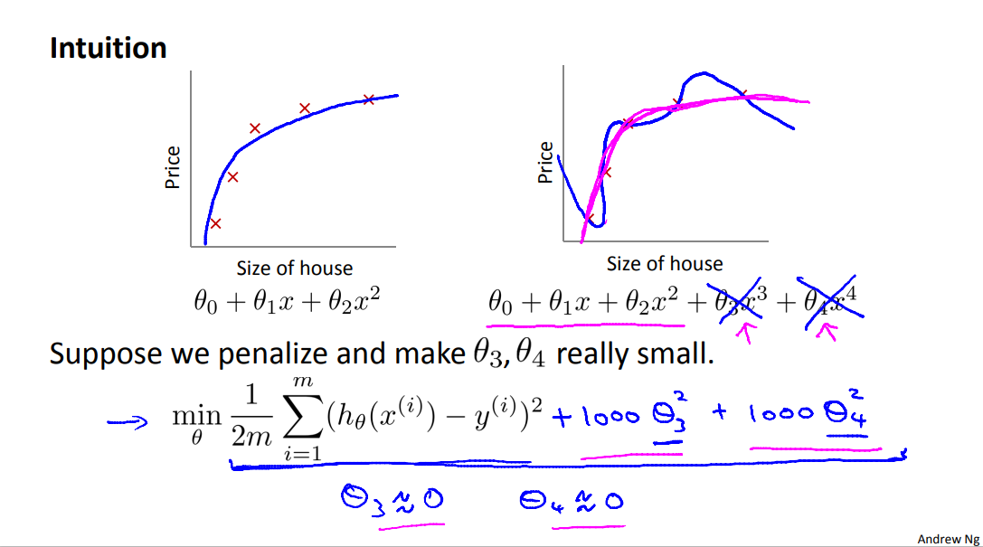
More generally, here is the idea behind regularization. The idea is that, if we have small values for the parameters, then, having small values for the parameters, will somehow, will usually correspond to having a simpler hypothesis. So, for our last example, we penalize just theta 3 and theta 4 and when both of these were close to zero, we wound up with a much simpler hypothesis that was essentially a quadratic function. it is possible to show that having smaller values of the parameters corresponds to usually smoother functions as well for the simpler.

Lets look at the specific example. For housing price prediction we may have our hundred features that we talked about where may be x1 is the size, x2 is the number of bedrooms, x3 is the number of floors and so on. And we may we may have a hundred features. And unlike the polynomial example, we don't know, right, we don't know that theta 3, theta 4, are the high order polynomial terms. So, if we have just a bag, if we have just a set of a hundred features, it's hard to pick in advance which are the ones that are less likely to be relevant. So we have a hundred or a hundred one parameters. And we don't know which ones to pick, we don't know which parameters to try to pick, to try to shrink.

So, in regularization, what we're going to do, is take our cost function, here's my cost function for linear regression. And what I'm going to do is, modify this cost function to shrink all of my parameters, because, you know, I don't know which one or two to try to shrink. So I am going to modify my cost function to add a term at the end. Like so we have square brackets here as well. When I add an extra regularization term at the end to shrink every single parameter and so this term we tend to shrink all of my parameters theta 1, theta 2, theta 3 up to theta 100.

$$mi{n}_{\theta }{\displaystyle \frac{1}{2m}}\sum _{i=1}^m(h_{\theta }(x^{(i)})-y^{(i)}{)}^2+\lambda \sum _{j=1}^n{\theta }_j^2$$

注意这里的cost function与后面给的线性回归梯度下降并不太匹配。不过核心思想是一致的。只不过是为了某些一致性，对于惩罚项做了修正，使得线性正则和逻辑正则的梯度下降看起来很一致。为了匹配下面的线性回归梯度下降，代价函数应修正为:

$$mi{n}_{\theta }{\displaystyle \frac{1}{2m}}\sum _{i=1}^m(h_{\theta }(x^{(i)})-y^{(i)}{)}^2+\frac{\lambda }{2m}\sum _{j=1}^n{\theta }_j^2$$

By the way, by convention the summation here starts from one so I am not actually going penalize theta zero being large. That sort of the convention that, the sum I equals one through N, rather than I equals zero through N. But in practice, it makes very little difference, and, whether you include, you know, theta zero or not, in practice, make very little difference to the results.

The λ, or lambda, is the regularization parameter. It determines how much the costs of our theta parameters are inflated.

It controls a trade off between two different goals. The first goal, capture it by the first goal objective, is that we would like to train, is that we would like to fit the training data well. We would like to fit the training set well. And the second goal is, we want to keep the parameters small, and that's captured by the second term, by the regularization objective. And by the regularization term. And what lambda, the regularization parameter does is the controls the trade of between these two goals, between the goal of fitting the training set well and the goal of keeping the parameter plan small and therefore keeping the hypothesis relatively simple to avoid overfitting.

Using the above cost function with the extra summation, we can smooth the output of our hypothesis function to reduce overfitting. If lambda is chosen to be too large, it may smooth out the function too much and cause underfitting. Hence, what would happen if $\lambda =0$ or is too small ?

And when we talk about multi-selection later in this course, we'll talk about a way, a variety of ways for automatically choosing the regularization parameter lambda as well.

unfamiliar words

1. eliminate
   英 [ɪˈlɪmɪneɪt] 美 [ɪˈlɪmɪneɪt]
   vt.
   排除;清除;消除;

2. inflated
   英 [ɪnˈfleɪtɪd] 美 [ɪnˈfleɪtɪd]
   adj.
   膨胀的;夸张的;

4.3 Regularized Linear Regression

Note: [8:43 - It is said that X is non-invertible if m ≤ n. The correct statement should be that X is non-invertible if m < n, and may be non-invertible if m = n.]

We can apply regularization to both linear regression and logistic regression. We will approach linear regression first.

Gradient Descent

We will modify our gradient descent function to separate out ${\theta }_0$ from the rest of the parameters because we do not want to penalize ${\theta }_0$.

$$\begin{array}{rl}& \text{Repeat}\{\\ & {\theta }_0:={\theta }_0-\alpha \frac{1}{m}\sum _{i=1}^m(h_{\theta }(x^{(i)})-y^{(i)})x_0^{(i)}\\ & {\theta }_j:={\theta }_j-\alpha [(\frac{1}{m}\sum _{i=1}^m(h_{\theta }(x^{(i)})-y^{(i)})x_j^{(i)})+\frac{\lambda }{m}{\theta }_j]& j\in \{1,2...n\}\\ & \}\end{array}$$

The term $\frac{\lambda }{m}{\theta }_j$ performs our regularization. With some manipulation our update rule can also be represented as:

$${\theta }_j:={\theta }_j(1-\alpha \frac{\lambda }{m})-\alpha \frac{1}{m}\sum _{i=1}^m(h_{\theta }(x^{(i)})-y^{(i)})x_j^{(i)}\theta$$

The first term in the above equation, $1-\alpha \frac{\lambda }{m}$ will always be less than 1. Intuitively you can see it as reducing the value of ${\theta }_j$ by some amount on every update. Notice that the second term is now exactly the same as it was before.

Normal Equation

Now let's approach regularization using the alternate method of the non-iterative normal equation.

To add in regularization, the equation is the same as our original, except that we add another term inside the parentheses:

$$\begin{array}{rl}& \theta ={(X^{T}X+\lambda \cdot L)}^{-1}{X}^{T}y\\ & \text{where}L=\left[\begin{array}{ccccc}0& & & & \\ & 1& & & \\ & & 1& & \\ & & & \ddots & \\ & & & & 1\end{array}\right]\end{array}$$

L is a matrix with 0 at the top left and 1's down the diagonal, with 0's everywhere else. It should have dimension (n+1)×(n+1). Intuitively, this is the identity matrix (though we are not including $x_0$ ), multiplied with a single real number λ.

Recall that if m < n, then $X^{T}X$ is non-invertible. However, when we add the term λ⋅L, then $X^{T}X$ + λ⋅L becomes invertible.

4.4 Regularized Logistic Regression

We can regularize logistic regression in a similar way that we regularize linear regression. As a result, we can avoid overfitting. The following image shows how the regularized function, displayed by the pink line, is less likely to overfit than the non-regularized function represented by the blue line:

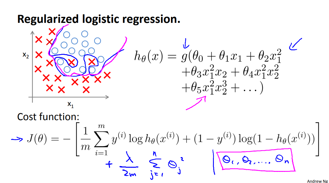
So, when we using regularization, even when you have a lot of features, the regularization can hel p take careof the overfitting probem.

Cost Function

Recall that our cost function for logistic regression was:

$$J(\theta )=-\frac{1}{m}\sum _{i=1}^m[y^{(i)}\log (h_{\theta }(x^{(i)}))+(1-y^{(i)})\log (1-h_{\theta }(x^{(i)}))]$$

We can regularize this equation by adding a term to the end:

$$J(\theta )=-\frac{1}{m}\sum _{i=1}^m[y^{(i)}\log (h_{\theta }(x^{(i)}))+(1-y^{(i)})\log (1-h_{\theta }(x^{(i)}))]+\frac{\lambda }{2m}\sum _{j=1}^n{\theta }_j^2$$

The second sum, $\sum _{j=1}^n{\theta }_j^2$ means to explicitly exclude the bias term, ${\theta }_0$. I.e. the θ vector is indexed from 0 to n (holding n+1 values, ${\theta }_0$ through ${\theta }_n$, and this sum explicitly skips ${\theta }_0$, by running from 1 to n, skipping 0. Thus, when computing the equation, we should continuously update the two following equations:

So, congratulations.

You've actually come a long ways. And you can actually, you actually know enough to apply this stuff and get to work for many problems.

So congratulations for that. But of course, there's still a lot more that we want to teach you, and in the next set of videos after this, we'll start to talk about a very powerful cause of non-linear classifier. So whereas linear regression, logistic regression, you know, you can form polynomial terms, but it turns out that there are much more powerful nonlinear quantifiers that can then sort of polynomial regression. And in the next set of videos after this one, I'll start telling you about them. So that you have even more powerful learning algorithms than you have now to apply to different problems.