Machine Learning Week_1 Parameter Learning 1-6

目录

• 3 Parameter Learning
  • 3.1 Video: Gradient Descent
    • unfamiliar words
  • 3.2 Reading：Gradient Descent
    • unfamiliar words
  • 3.3 Video: Gradient Descent Intuition
    • unfamiliar words
  • 3.4 Reading: Gradient Descent Intuition
    • unfamiliar words
  • 3.5 Video: Gradient Descent For Linear Regression
    • unfamiliar words
  • 3.6 Reading: Gradient Descent For Linear Regression
    • unfamiliar words

3 Parameter Learning

3.1 Video: Gradient Descent

We previously defined the cost function J.

In this video, I want to tell you about an algorithm called gradient descent for minimizing the cost function J. It turns out gradient descent is a more general algorithm, and is used not only in linear regression. It's actually used all over the place in machine learning. And later in the class, we'll use gradient descent to minimize other functions as well, not just the cost function J for the linear regression.

So in this video, we'll talk about gradient descent for minimizing some arbitrary function J and then in later videos, we'll take this algorithm and apply it specifically to the cost function J that we have defined for linear regression.

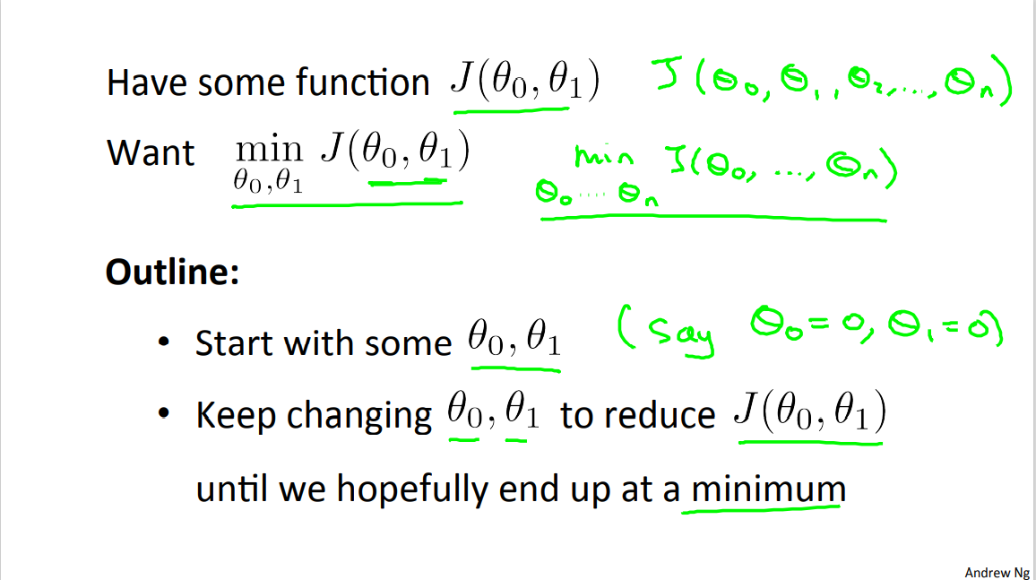
So here's the problem setup. Going to assume that we have some function J(theta 0, theta 1) maybe it's the cost function from linear regression, maybe it's some other function we wanna minimize. And we want to come up with an algorithm for minimizing that as a function of J(theta 0, theta 1). Just as an aside it turns out that gradient descent actually applies to more general functions. So imagine, if you have a function that's a function of J, as theta 0, theta 1, theta 2, up to say some theta n, and you want to minimize theta 0. You minimize over theta 0 up to theta n of this J of theta 0 up to theta n. And it turns our gradient descent is an algorithm for solving this more general problem. But for the sake of brevity, for the sake of succinctness of notation, I'm just going to pretend I have only two parameters throughout the rest of this video. Here's the idea for gradient descent. What we're going to do is we're going to start off with some initial guesses for theta 0 and theta 1. Doesn't really matter what they are, but a common choice would be we set theta 0 to 0, and set theta 1 to 0, just initialize them to 0. What we're going to do in gradient descent is we'll keep changing theta 0 and theta 1 a little bit to try to reduce J(theta 0, theta 1), until hopefully, we wind at a minimum, or maybe at a local minimum.

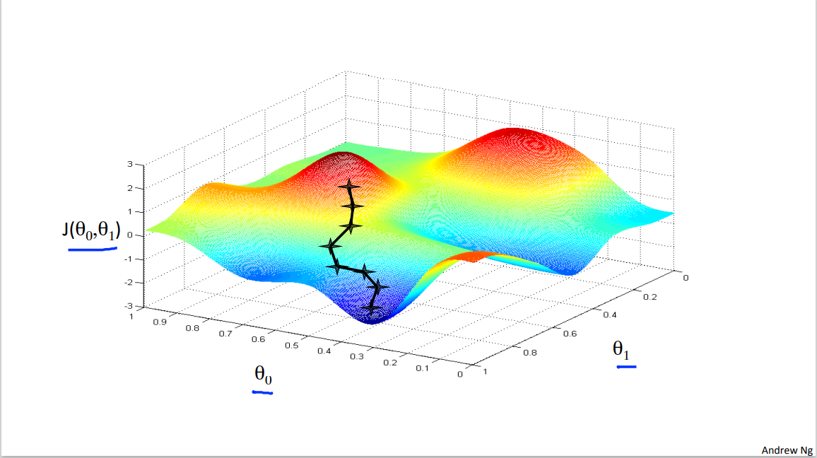
So let's see in pictures what gradient descent does. Let's say you're trying to minimize this function. So notice the axes, this is theta 0, theta 1 on the horizontal axes and J is the vertical axis and so the height of the surface shows J and we want to minimize this function. So we're going to start off with theta 0, theta 1 at some point. So imagine picking some value for theta 0, theta 1, and that corresponds to starting at some point on the surface of this function. So whatever value of theta 0, theta 1 gives you some point here. I did initialize them to 0, 0 but sometimes you initialize it to other values as well.

Now, I want you to imagine that this figure shows a hole. Imagine this is like the landscape of some grassy park, with two hills like so, and I want us to imagine that you are physically standing at that point on the hill, on this little red hill in your park. In gradient descent, what we're going to do is we're going to spin 360 degrees around, just look all around us, and ask, if I were to take a little baby step in some direction, and I want to go downhill as quickly as possible, what direction do I take that little baby step in? If I wanna go down, so I wanna physically walk down this hill as rapidly as possible.

Turns out, that if you're standing at that point on the hill, you look all around and you find that the best direction is to take a little step downhill is roughly that direction. Okay, and now you're at this new point on your hill. You're gonna, again, look all around and say what direction should I step in order to take a little baby step downhill? And if you do that and take another step, you take a step in that direction.

And then you keep going. From this new point you look around, decide what direction would take you downhill most quickly. Take another step, another step, and so on until you converge to this local minimum down here.

Gradient descent has an interesting property.

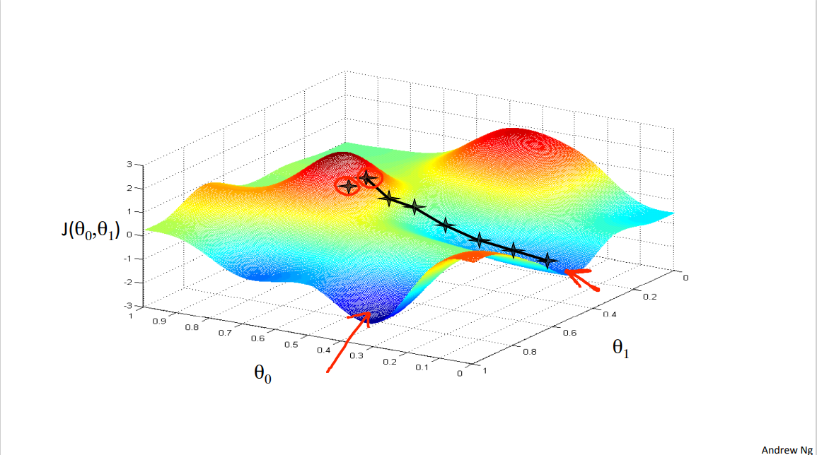
This first time we ran gradient descent we were starting at this point over here, right? Started at that point over here. Now imagine we had initialized gradient descent just a couple steps to the right. Imagine we'd initialized gradient descent with that point on the upper right. If you were to repeat this process, so start from that point, look all around, take a little step in the direction of steepest descent, you would do that. Then look around, take another step, and so on.

And if you started just a couple of steps to the right, gradient descent would've taken you to this second local optimum over on the right.

So if you had started this first point, you would've wound up at this local optimum, but if you started just at a slightly different location, you would've wound up at a very different local optimum. And this is a property of gradient descent that we'll say a little bit more about later. So that's the intuition in pictures.

Let's look at the math. This is the definition of the gradient descent algorithm. We're going to just repeatedly do this until convergence, we're going to update my parameter theta j by taking theta j and subtracting from it alpha times this term over here, okay? So let's see, there's lot of details in this equation so let me unpack some of it. First, this notation here, :=, gonna use := to denote assignment, so it's the assignment operator. So briefly, if I write a := b, what this means is, it means in a computer, this means take the value in b and use it overwrite whatever value is a. So this means set a to be equal to the value of b, which is assignment. And I can also do a := a + 1. This means take a and increase its value by one. Whereas in contrast, if I use the equal sign and I write a equals b, then this is a truth assertion.

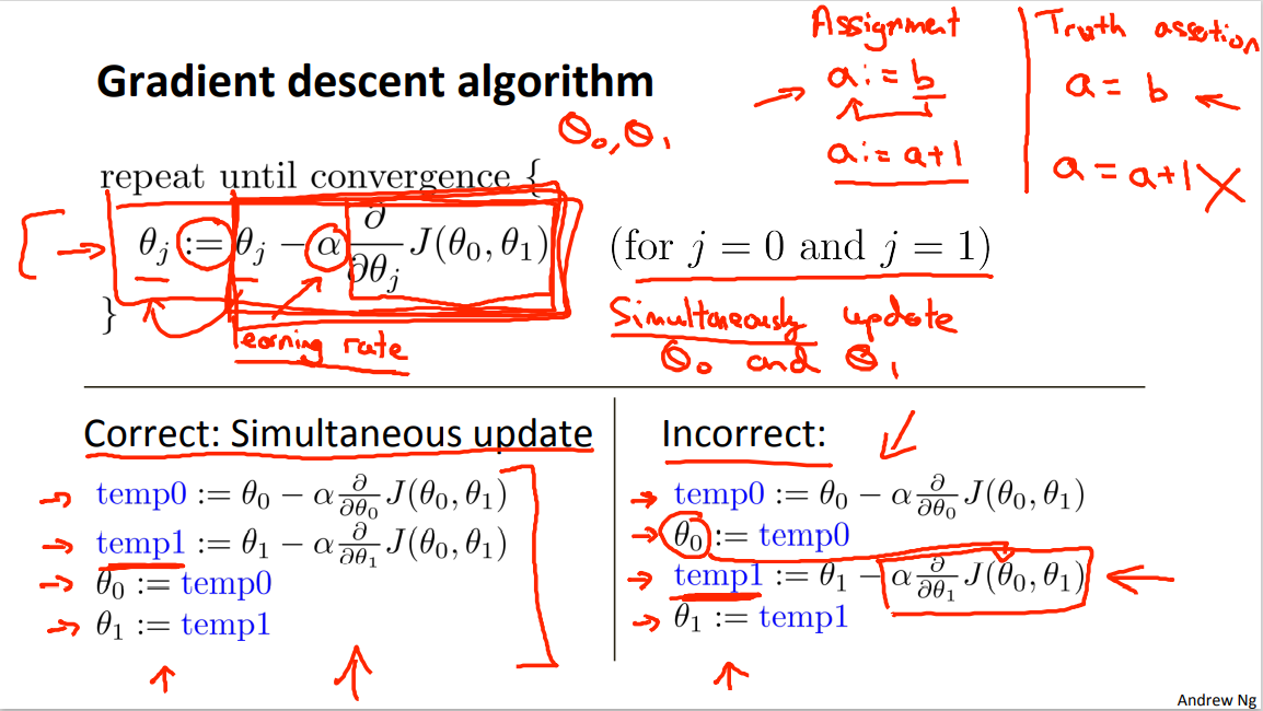
Okay? So if I write a equals b, then I'll asserting that the value of a equals to the value of b, right? So the left hand side, that's the computer operation, where we set the value of a to a new value. The right hand side, this is asserting, I'm just making a claim that the values of a and b are the same, and so whereas you can write a := a + 1, that means increment a by 1, hopefully I won't ever write a = a + 1 because that's just wrong. a and a + 1 can never be equal to the same values. Okay? So this is first part of the definition. This alpha here is a number that is called the learning rate.

And what alpha does is it basically controls how big a step we take downhill with creating descent. So if alpha is very large, then that corresponds to a very aggressive gradient descent procedure where we're trying take huge steps downhill and if alpha is very small, then we're taking little, little baby steps downhill. And I'll come back and say more about this later, about how to set alpha and so on.

And finally, this term here, that's a derivative term. I don't wanna talk about it right now, but I will derive this derivative term and tell you exactly what this is later, okay? And some of you will be more familiar with calculus than others, but even if you aren't familiar with calculus, don't worry about it. I'll tell you what you need to know about this term here.

Now, there's one more subtlety about gradient descent which is in gradient descent we're going to update, you know, theta 0 and theta 1, right? So this update takes place for j = 0 and j = 1, so you're gonna update theta 0 and update theta 1. And the subtlety of how you implement gradient descent is for this expression, for this update equation, you want to simultaneously update theta 0 and theta 1. What I mean by that is that in this equation, we're gonna update theta 0 := theta 0 minus something, and update theta 1 := theta 1 minus something. And the way to implement is you should compute the right hand side, right? Compute that thing for theta 0 and theta 1 and then simultaneously, at the same time, update theta 0 and theta 1, okay? So let me say what I mean by that. This is a correct implementation of gradient descent meaning simultaneous update. So I'm gonna set temp0 equals that, set temp1 equals that so basic compute the right-hand sides, and then having computed the right-hand sides and stored them into variables temp0 and temp1, I'm gonna update theta 0 and theta 1 simultaneously because that's the correct implementation.

In contrast, here's an incorrect implementation that does not do a simultaneous update. So in this incorrect implementation, we compute temp0, and then we update theta 0, and then we compute temp1, and then we update temp1.

And the difference between the right hand side and the left hand side implementations is that If you look down here, you look at this step, if by this time you've already updated theta 0, then you would be using the new value of theta 0 to compute this derivative term. And so this gives you a different value of temp1, than the left-hand side, right? Because you've now plugged in the new value of theta 0 into this equation. And so, this on the right-hand side is not a correct implementation of gradient descent, okay? So I don't wanna say why you need to do the simultaneous updates. It turns out that the way gradient descent is usually implemented, which I'll say more about later, it actually turns out to be more natural to implement the simultaneous updates.

And when people talk about gradient descent, they always mean simultaneous update. If you implement the non simultaneous update, it turns out it will probably work anyway. But this algorithm wasn't right. It's not what people refer to as gradient descent, and this is some other algorithm with different properties. And for various reasons this can behave in slightly stranger ways, and so what you should do is really implement the simultaneous update of gradient descent. So, that's the outline of the gradient descent algorithm.

In the next video, we're going to go into the details of the derivative term, which I wrote up but didn't really define. And if you've taken a calculus class before and if you're familiar with partial derivatives and derivatives, it turns out that's exactly what that derivative term is, but in case you aren't familiar with calculus, don't worry about it. The next video will give you all the intuitions and will tell you everything you need to know to compute that derivative term, even if you haven't seen calculus, or even if you haven't seen partial derivatives before.

And with that, with the next video, hopefully we'll be able to give you all the intuitions you need to apply gradient descent.

unfamiliar words

we'll talk about gradient descent for minimizing some arbitrary function J
Just as an aside it turns out that gradient descent actually applies to more general functions.
But for the sake of brevity.
for the sake of succinctness of notation.
Imagine this is like the landscape of some grassy park, with two hills like so.
In gradient descent, what we're going to do is we're going to spin 360 degrees around, just look all around us.
Take another step, another step, and so on until you converge to this local minimum down here.
So if you had started this first point, you would've wound up at this local optimum.
So let's see, there's lot of details in this equation so let me unpack some of it.
if I use the equal sign and I write a equals b, then this is a truth assertion.
And what alpha does is it basically controls how big a step we take downhill with creating descent. So if alpha is very large, then that corresponds to a very aggressive gradient descent procedure.
And finally, this term here, that's a derivative term.
Now, there's one more subtlety about gradient descent which is in gradient descent we're going to update.
you want to simultaneously update theta 0 and theta 1.
So, that's the outline of the gradient descent algorithm.

3.2 Reading：Gradient Descent

So we have our hypothesis function and we have a way of measuring how well it fits into the data. Now we need to estimate the parameters in the hypothesis function. That's where gradient descent comes in.

Imagine that we graph our hypothesis function based on its fields \(\theta_0\) and \(\theta_1\) (actually we are graphing the cost function as a function of the parameter estimates). We are not graphing x and y itself, but the parameter range of our hypothesis function and the cost resulting from selecting a particular set of parameters.

We put \(\theta_0\) on the x axis and \(\theta_1\) on the y axis, with the cost function on the vertical z axis. The points on our graph will be the result of the cost function using our hypothesis with those specific theta parameters. The graph below depicts such a setup.

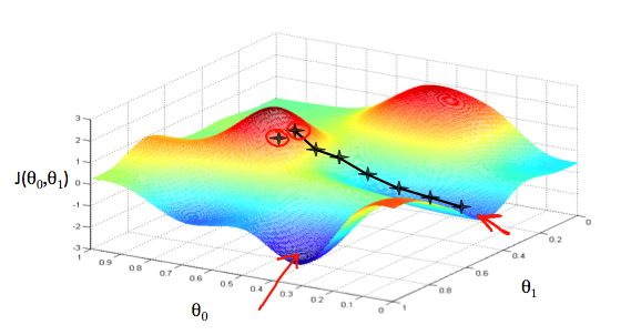
We will know that we have succeeded when our cost function is at the very bottom of the pits in our graph, i.e. when its value is the minimum. The red arrows show the minimum points in the graph.

The way we do this is by taking the derivative (the tangential line to a function) of our cost function. The slope of the tangent is the derivative at that point and it will give us a direction to move towards. We make steps down the cost function in the direction with the steepest descent. The size of each step is determined by the parameter α, which is called the learning rate.

For example, the distance between each 'star' in the graph above represents a step determined by our parameter α. A smaller α would result in a smaller step and a larger α results in a larger step. The direction in which the step is taken is determined by the partial derivative of \(J(\theta_{0},\theta_{1})\). Depending on where one starts on the graph, one could end up at different points. The image above shows us two different starting points that end up in two different places.

The gradient descent algorithm is:

repeat until convergence:

\( \theta_j := \theta_j - \alpha \frac{\partial}{\partial \theta_j} J(\theta_0, \theta_1) \)

where

j=0,1 represents the feature index number.

At each iteration j, one should simultaneously update the parameters \(\theta_1, \theta_2,...,\theta_n\). Updating a specific parameter prior to calculating another one on the \(j^{(th)}\) iteration would yield to a wrong implementation.

unfamiliar words

The graph below depicts such a setup.
We will know that we have succeeded when our cost function is at the very bottom of the pits in our graph
the tangential line to a function
We make steps down the cost function in the direction with the steepest descent.
Updating a specific parameter prior to calculating another one on the \(j^{(th)}\) iteration would yield to a wrong implementation.

3.3 Video: Gradient Descent Intuition

In the previous video, we gave a mathematical definition of gradient descent. Let's delve deeper and in this video get better intuition about what the algorithm is doing and why the steps of the gradient descent algorithm might make sense.

Here's a gradient descent algorithm that we saw last time and just to remind you this parameter, or this term alpha is called the learning rate. And it controls how big a step we take when updating my parameter theta j.

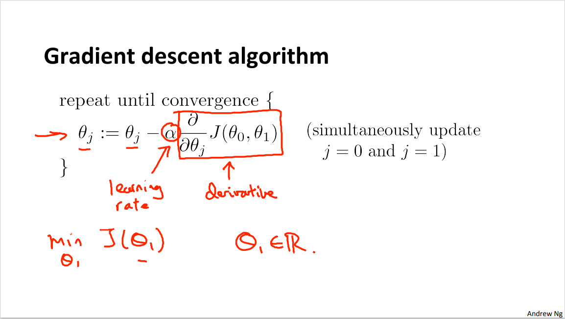
And this second term here is the derivative term.

And what I wanna do in this video is give you that intuition about what each of these two terms is doing and why when put together, this entire update makes sense. In order to convey these intuitions, what I want to do is use a slightly simpler example, where we want to minimize the function of just one parameter. So say we have a cost function, j of just one parameter, theta one, like we did a few videos back, where theta one is a real number. So we can have 1D(one-dimensional) plots, which are a little bit simpler to look at. Let's try to understand what gradient decent would do on this function.

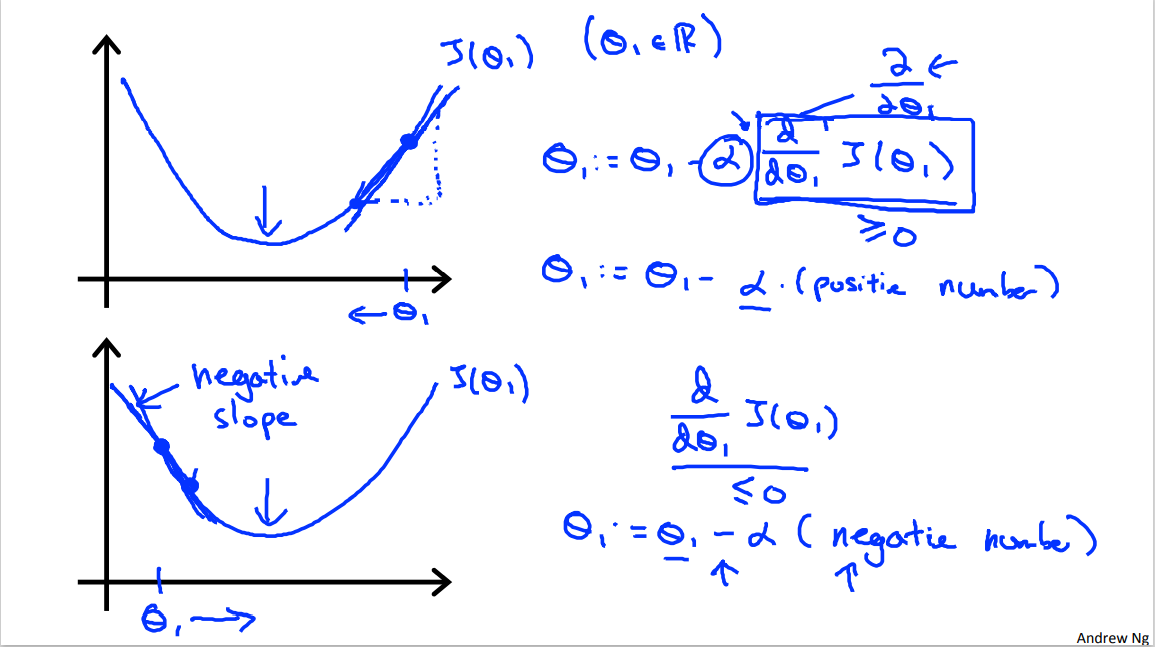
So let's say, here's my function, J of theta 1. And so that's mine. And where theta 1 is a real number. All right? Now, let's have in this slide its grade in descent with theta one at this location. So imagine that we start off at that point on my function.

What grade in descent would do is it will update.

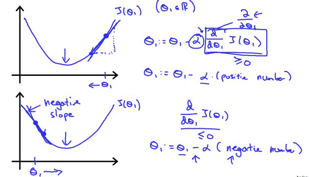
Theta one gets updated as theta one minus alpha times d d theta one J of theta one, right? And as an aside, this derivative term, right, if you're wondering why I changed the notation from these partial derivative symbols. If you don't know what the difference is between these partial derivative symbols and the dd theta, don't worry about it. Technically in mathematics you call this a partial derivative and call this a derivative, depending on the number of parameters in the function J. But that's a mathematical technicality. And so for the purpose of this lecture, think of these partial symbols and d, d theta 1, as exactly the same thing. And don't worry about what the real difference is. I'm gonna try to use the mathematically precise notation, but for our purposes these two notations are really the same thing. And so let's see what this equation will do. So we're going to compute this derivative, not sure if you've seen derivatives in calculus before, but what the derivative at this point does, is basically saying, now let's take the tangent to that point, like that straight line, that red line, is just touching this function, and let's look at the slope of this red line. That's what the derivative is, it's saying what's the slope of the line that is just tangent to the function. Okay, the slope of a line is just this height divided by this horizontal thing. Now, this line has a positive slope, so it has a positive derivative. And so my update to theta is going to be theta 1, it gets updated as theta 1, minus alpha times some positive number.

Okay. Alpha the the learning, is always a positive number. And, so we're going to take theta one is updated as theta one minus something. So I'm gonna end up moving theta one to the left. I'm gonna decrease theta one, and we can see this is the right thing to do cuz I actually wanna head in this direction. You know, to get me closer to the minimum over there.

So, gradient descent so far says we're going the right thing. Let's look at another example. So let's take my same function J, let's try to draw from the same function, J of theta 1. And now, let's say I had to say initialize my parameter over there on the left. So theta 1 is here. I glare at that point on the surface.

Now my derivative term, d/d theta one J of theta one when you value into that this point, we're gonna look at right the slope of that line, so this derivative term is a slope of this line. But this line is slanting down, so this line has negative slope.

Right. Or alternatively, I say that this function has negative derivative, just means negative slope at that point. So this is less than equals to 0, so when I update theta, I'm gonna have theta. Just update this theta of minus alpha times a negative number.

And so I have theta 1 minus a negative number which means I'm actually going to increase theta, because it's minus of a negative number, means I'm adding something to theta. And what that means is that I'm going to end up increasing theta until it's not here, and increase theta wish again seems like the thing I wanted to do to try to get me closer to the minimum.

So this whole theory of intuition behind what a derivative is doing, let's take a look at the rate term alpha and see what that's doing.

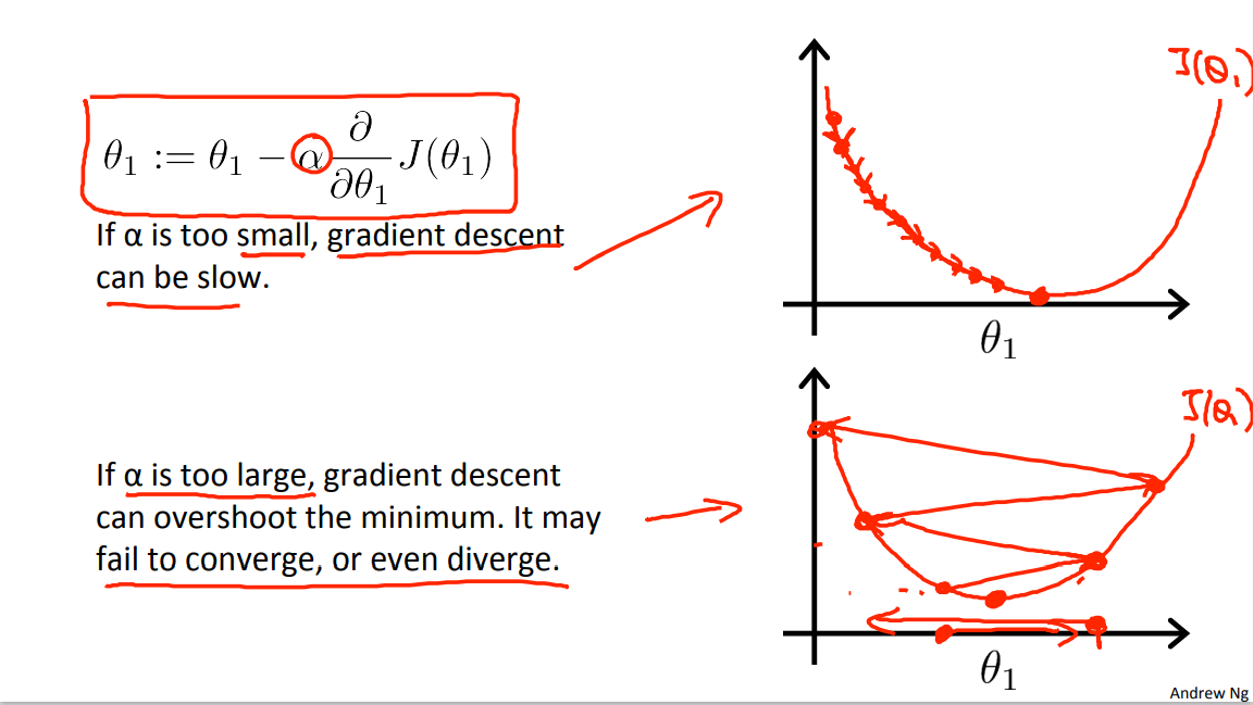
So here's my gradient descent update rule, that's this equation.

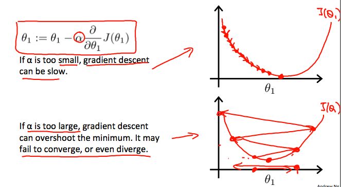
And let's look at what could happen if alpha is either too small or if alpha is too large. So this first example, what happens if alpha is too small? So here's my function J, J of theta. Let's all start here. If alpha is too small, then what I'm gonna do is gonna multiply my update by some small number, so end up taking a baby step like that. Okay, so this one step. Then from this new point, I'm gonna have to take another step. But if alpha's too small, I take another little baby step. And so if my learning rate is too small I'm gonna end up taking these tiny tiny baby steps as you try to get to the minimum. And I'm gonna need a lot of steps to get to the minimum and so if alpha is too small gradient descent can be slow because it's gonna take these tiny tiny baby steps and so it's gonna need a lot of steps before it gets anywhere close to the global minimum.

Now how about if our alpha is too large? So, here's my function J of theta, turns out of that alpha's too large, then gradient descent can overshoot the minimum and may even fail to convert or even divert, so here's what I mean. Let's say a start of data there, it's actually close to minimum. So the derivative points to the right, but if alpha is too big, I'm gonna take a huge step. Remember, take a huge step like that. So it ends up taking a huge step, and now my cost functions has got worse. Cause it starts off with this value, and now, my values hasgot worse. Now my derivative points to the left, it's actually decrease theta. But look, if my learning is too big, I may take a huge step going from here all the way to out there. So we end up being over there, right? And if my learning rate is too big, we can take another huge step on the next iteration and kind of overshoot and overshoot and so on, until you already notice I'm actually getting further and further away from the minimum. So if alpha is to large, it can fail to converge or even diverge.

Now, I have another question for you. So this a tricky one and when I was first learning this stuff it actually took me a long time to figure this out. What if your parameter theta 1 is already at a local minimum, what do you think one step of gradient descent will do?

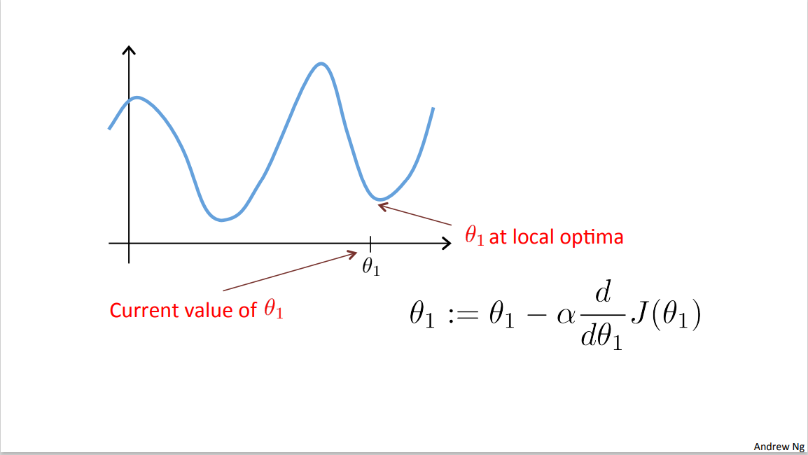
So let's suppose you initialize theta 1 at a local minimum. So, suppose this is your initial value of theta 1 over here and is already at a local optimum or the local minimum.

It turns out the local optimum, your derivative will be equal to zero. So for that slope, that tangent point, so the slope of this line will be equal to zero and thus this derivative term is equal to zero. And so your gradient descent update, you have theta one cuz I updated this theta one minus alpha times zero. And so what this means is that if you're already at the local optimum, it leaves theta 1 unchanged cause its updates as theta 1 equals theta 1. So if your parameters are already at a local minimum one step with gradient descent does absolutely nothing it doesn't change your parameter, which is, what you want because it keeps your solution at the local optimum.

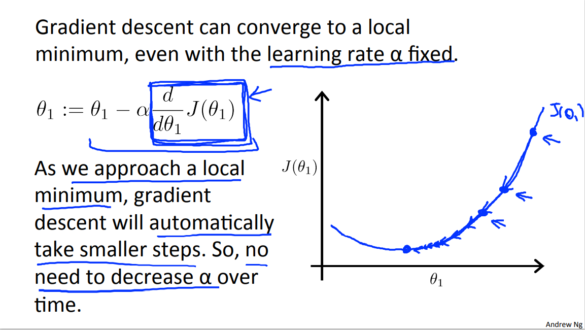
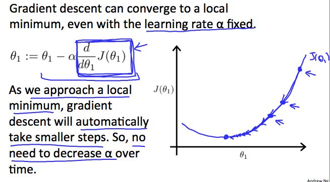
This also explains why gradient descent can converse the local minimum even with the learning rate alpha fixed. Here's what I mean by that let's look in the example. So here's a cost function J of theta that maybe I want to minimize and let's say I initialize my algorithm, my gradient descent algorithm, out there at that magenta point. If I take one step in gradient descent, maybe it will take me to that point, because my derivative's pretty steep out there. Right? Now, I'm at this green point, and if I take another step in gradient descent, you notice that my derivative, meaning the slope, is less steep at the green point than compared to at the magenta point out there. Because as I approach the minimum, my derivative gets closer and closer to zero, as I approach the minimum. So after one step of descent, my new derivative is a little bit smaller. So I wanna take another step in the gradient descent. I will naturally take a somewhat smaller step from this green point right there from the magenta point. Now with a new point, a red point, and I'm even closer to global minimum so the derivative here will be even smaller than it was at the green point. So I'm gonna another step in the gradient descent.

Now, my derivative term is even smaller and so the magnitude of the update to theta one is even smaller, so take a small step like so. And as gradient descent runs, you will automatically take smaller and smaller steps.

Until eventually you're taking very small steps, you know, and you finally converge to the to the local minimum.

So just to recap, in gradient descent as we approach a local minimum, gradient descent will automatically take smaller steps. And that's because as we approach the local minimum, by definition the local minimum is when the derivative is equal to zero. As we approach local minimum, this derivative term will automatically get smaller, and so gradient descent will automatically take smaller steps. This is what so no need to decrease alpha or the time.

So that's the gradient descent algorithm and you can use it to try to minimize any cost function J, not the cost function J that we defined for linear regression. In the next video, we're going to take the function J and set that back to be exactly linear regression's cost function, the square cost function that we came up with earlier. And taking gradient descent and the square cost function and putting them together. That will give us our first learning algorithm, that'll give us a linear regression algorithm.

unfamiliar words

In order to convey these intuitions
But this line is slanting down, so this line has negative slope.
Now, my derivative term is even smaller and so the magnitude of the update to theta one is even smaller

3.4 Reading: Gradient Descent Intuition

In this video we explored the scenario where we used one parameter \(\theta_1\) and plotted its cost function to implement a gradient descent. Our formula for a single parameter was :

Repeat until convergence:

\[\theta_1 := \theta_1 - \alpha \frac{\partial}{\partial \theta_1} J( \theta_1) \]

Regardless of the slope's sign for \(\frac{d}{d\theta_1} J(\theta_1)\), \(\theta_1\) eventually converges to its minimum value. The following graph shows that when the slope is negative, the value of \(\theta_1\) increases and when it is positive, the value of \(\theta_1\) decreases.

On a side note, we should adjust our parameter \(\alpha\) to ensure that the gradient descent algorithm converges in a reasonable time. Failure to converge or too much time to obtain the minimum value imply that our step size is wrong.

How does gradient descent converge with a fixed step size α?

The intuition behind the convergence is that \(\frac{d}{d\theta_1} J(\theta_1)\) approaches 0 as we approach the bottom of our convex function. At the minimum, the derivative will always be 0 and thus we get:

\[\theta_1:=\theta_1-\alpha * 0 \]

unfamiliar words

Failure to converge or too much time to obtain the minimum value imply that our step size is wrong.

3.5 Video: Gradient Descent For Linear Regression

In previous videos, we talked about the gradient descent algorithm and we talked about the linear regression model and the squared error cost function. In this video we're gonna put together gradient descent with our cost function, and that will give us an algorithm for linear regression or putting a straight line to our data.

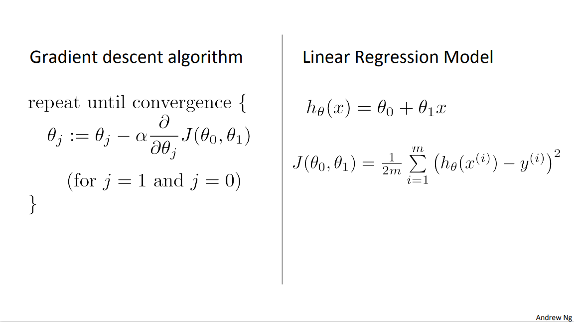
So this was what we worked out in the previous videos. This gradient descent algorithm which you should be familiar and here's the linear regression model with our linear hypothesis and our squared error cost function. What we're going to do is apply gradient descent to minimize our squared error cost function. Now in order to apply gradient descent, in order to, you know, write this piece of code, the key term we need is this derivative term over here. So you need to figure out what is this partial derivative term and plugging in the definition of the cause function j. This turns out to be this \(\frac{\partial}{\partial \theta_1} \frac{1}{2m}\).

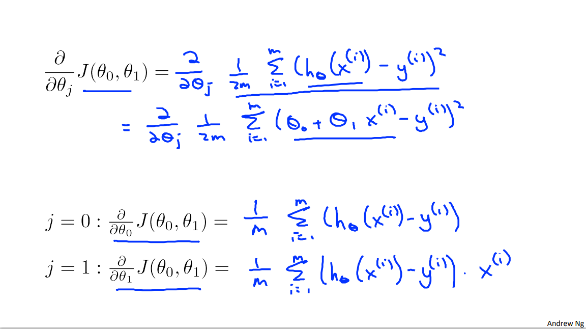
Something might equals 1 though m. Of this squared error cost function term. And all I did here was I just, you know plug in the definition of the cost function there.

And simplifying a little bit more, this turns out to be equal to this. Something equals one through m of theta zero plus theta one x i minus y i squared. And all I did there was I took the definition for my hypothesis and plugged it in there. And turns out we need to figure out what is this partial derivative for two cases for J equals 0 and J equals 1.

So we want to figure out what is this partial derivative for both the theta 0 case and the theta 1 case. And I'm just going to write out the answers. It turns out this first term is, simplifies to 1/M sum from over my training set of just that of x(i)- y(i) and for this term partial derivative let's write the theta 1, it turns out I get this term. ... Minus y(i) times x(i). Okay and computing these partial derivatives, so we're going from this equation. Right going from this equation to either of the equations down there. Computing those partial derivative terms requires some multivariate calculus. If you know calculus, feel free to work through the derivations yourself and check that if you take the derivatives, you actually get the answers that I got. But if you're less familiar with calculus, don't worry about it and it's fine to just take these equations that were worked out and you won't need to know calculus or anything like that, in order to do the homework so let's implement gradient descent and get back to work.

So armed with these definitions or armed with what we worked out to be the derivatives which is really just the slope of the cost function j.

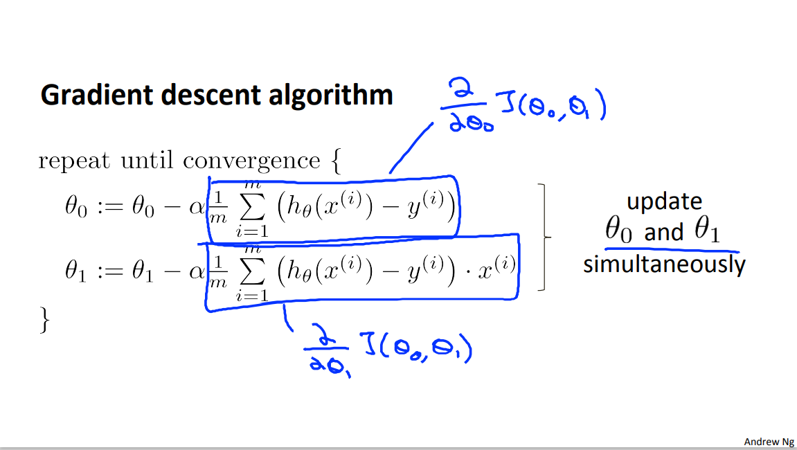
we can now plug them back in to our gradient descent algorithm. So here's gradient descent for linear regression which is gonna repeat until convergence, theta 0 and theta 1 get updated as you know this thing minus alpha times the derivative term.

So this term here.

So here's our linear regression algorithm.

This first term here.

That term is of course just the partial derivative with respect to theta zero, that we worked out on a previous slide. And this second term here, that term is just a partial derivative in respect to theta 1, that we worked out on the previous line. And just as a quick reminder, you must, when implementing gradient descent. There's actually this detail that you should be implementing it so the update theta 0 and theta 1 simultaneously.

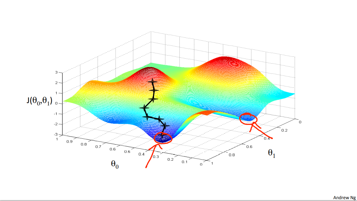
So. Let's see how gradient descent works. One of the issues we saw with gradient descent is that it can be susceptible to local optima. So when I first explained gradient descent I showed you this picture of it going downhill on the surface, and we saw how depending on where you initialize it, you can end up at different local optima. You will either wind up here or here.

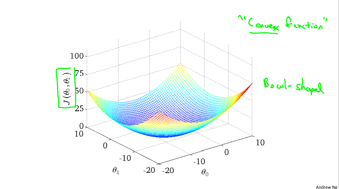
But, it turns out that that the cost function for linear regression is always going to be a bow shaped function like this. The technical term for this is that this is called a convex function.

And I'm not gonna give the formal definition for what is a convex function, C, O, N, V, E, X. But informally a convex function means a bowl shaped function and so this function doesn't have any local optima except for the one global optimum. And does gradient descent on this type of cost function which you get whenever you're using linear regression it will always converge to the global optimum. Because there are no other local optimum, just global optimum.

So now let's see this algorithm in action.

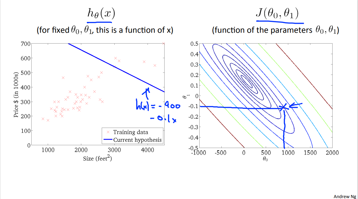
As usual, here are plots of the hypothesis function and of my cost function j. And so let's say I've initialized my parameters at this value. Let's say, usually you initialize your parameters at zero, zero. Theta zero and theta equals zero. But for the demonstration, in this physical infrontation I've initialized you know, theta zero at 900 and theta one at about -0.1 okay. And so this corresponds to h(x)=-900-0.1x, [the intercept should be +900] is this line, out here on the cost function.

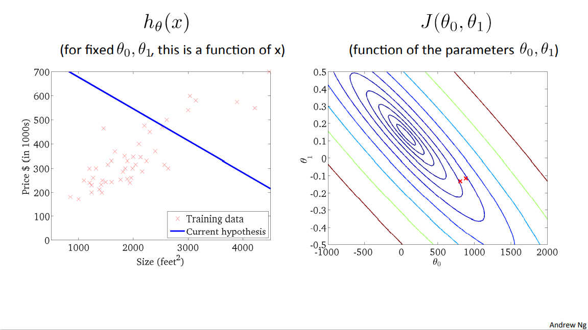
Now, if we take one step in gradient descent, we end up going from this point out here, over to the down and left, to that second point over there. And you notice that my line changed a little bit, and as I take another step of gradient descent, my line on the left will change.

Right? And I've also moved to a new point on my cost function.

And as I take further steps of gradient descent, I'm going down in cost. So my parameters and such are following this trajectory.

And if you look on the left, this corresponds with hypotheses. That seem to be getting to be better and better fits to the data.

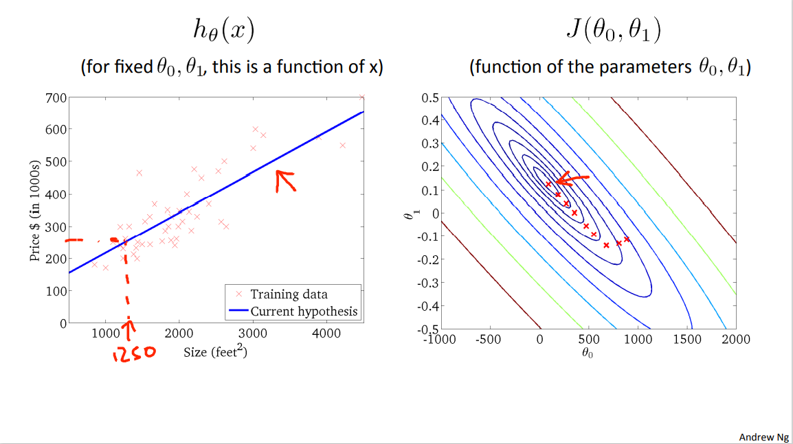
until eventually I've now wound up at the global minimum and this global minimum corresponds to this hypothesis, which gets me a good fit to the data.

And so that's gradient descent, and we've just run it and gotten a good fit to my data set of housing prices. And you can now use it to predict, you know, if your friend has a house size 1250 square feet, you can now read off the value and tell them that I don't know maybe they could get $250,000 for their house.

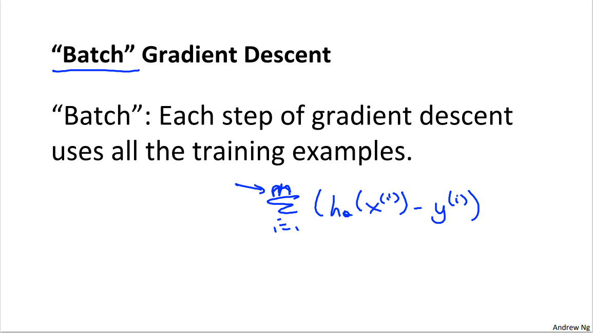
Finally just to give this another name it turns out that the algorithm that we just went over is sometimes called batch gradient descent. And it turns out in machine learning I don't know I feel like us machine learning people were not always great at giving names to algorithms. But the term batch gradient descent refers to the fact that in every step of gradient descent, we're looking at all of the training examples. So in gradient descent, when computing the derivatives, we're computing the sums [INAUDIBLE]. So ever step of gradient descent we end up computing something like this that sums over our m training examples and so the term batch gradient descent refers to the fact that we're looking at the entire batch of training examples. And again, it's really not a great name, but this is what machine learning people call it. And it turns out that there are sometimes other versions of gradient descent that are not batch versions, but they are instead. Do not look at the entire training set but look at small subsets of the training sets at a time. And we'll talk about those versions later in this course as well. But for now using the algorithm we just learned about or using batch gradient descent you now know how to implement gradient descent for linear regression.

So that's linear regression with gradient descent. If you've seen advanced linear algebra before, so some of you may have taken a class in advanced linear algebra. You might know that there exists a solution for numerically solving for the minimum of the cost function j without needing to use an iterative algorithm like gradient descent. Later in this course we'll talk about that method as well that just solves for the minimum of the cost function j without needing these multiple steps of gradient descent. That other method is called the normal equations method. But in case you've heard of that method it turns out that gradient descent will scale better to larger data sets than that normal equation method. And now that we know about gradient descent we'll be able to use it in lots of different contexts and we'll use it in lots of different machine learning problems as well.

So congrats on learning about your first machine learning algorithm. We'll later have exercises in which we'll ask you to implement gradient descent and hopefully see these algorithms right for yourselves. But before that I first want to tell you in the next set of videos. The first one to tell you about a generalization of the gradient descent algorithm that will make it much more powerful. And I guess I'll tell you about that in the next video.

unfamiliar words

So armed with these definitions or armed with what we worked out to be the derivatives which is really just the slope of the cost function j.
So my parameters and such are following this trajectory.

3.6 Reading: Gradient Descent For Linear Regression

When specifically applied to the case of linear regression, a new form of the gradient descent equation can be derived. We can substitute our actual cost function and our actual hypothesis function and modify the equation to :

where m is the size of the training set, \(\theta_0\) a constant that will be changing simultaneously with \(\theta_1\) and \(x_{i}, y_{i}\) are values of the given training set (data).

Note that we have separated out the two cases for \(\theta_j\) into separate equations for \(\theta_0\) and \(\theta_1\) and that for \(\theta_1\) we are multiplying \(x_{i}\) at the end due to the derivative. The following is a derivation of \(\frac {\partial}{\partial \theta_j}J(\theta)\) for a single example :

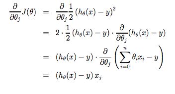
The point of all this is that if we start with a guess for our hypothesis and then repeatedly apply these gradient descent equations, our hypothesis will become more and more accurate.

So, this is simply gradient descent on the original cost function J. This method looks at every example in the entire training set on every step, and is called batch gradient descent. Note that, while gradient descent can be susceptible to local minima in general, the optimization problem we have posed here for linear regression has only one global, and no other local, optima; thus gradient descent always converges (assuming the learning rate α is not too large) to the global minimum. Indeed, J is a convex quadratic function. Here is an example of gradient descent as it is run to minimize a quadratic function.

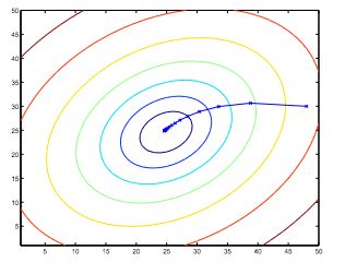
The ellipses shown above are the contours of a quadratic function. Also shown is the trajectory taken by gradient descent, which was initialized at (48,30). The x’s in the figure (joined by straight lines) mark the successive values of θ that gradient descent went through as it converged to its minimum.

unfamiliar words