PointNetCFD-main

##### Point-cloud deep learning for prediction of fluid flow fields on irregular geometries (supervised learning) #####

#Authors: Ali Kashefi (kashefi@stanford.edu) and Davis Rempe (drempe@stanford.edu)
#Description: Implementation of PointNet for *supervised learning* of computational mechanics on domains with irregular geometries
#Version: 1.0
#Guidance: We recommend opening and running the code on **[Google Colab](https://research.google.com/colaboratory)** as a first try. 

##### Citation #####
#If you use the code, please cite the following journal paper: 
#[A point-cloud deep learning framework for prediction of fluid flow fields on irregular geometries]
#(https://aip.scitation.org/doi/full/10.1063/5.0033376)

#@article{kashefi2021PointNetCFD, 
#author = {Kashefi, Ali  and Rempe, Davis  and Guibas, Leonidas J. }, 
#title = {A point-cloud deep learning framework for prediction of fluid flow fields on irregular geometries}, 
#journal = {Physics of Fluids}, 
#volume = {33}, 
#number = {2}, 
#pages = {027104}, 
#year = {2021}, 
#doi = {10.1063/5.0033376},}

##### Importing libraries #####
#As a first step, we import the necessary libraries.
#We use [Matplotlib](https://matplotlib.org/) for visualization purposes and [NumPy](https://numpy.org/) for computing on arrays.

import os
import linecache
import math
from operator import itemgetter
import numpy as np
from numpy import zeros
import matplotlib
matplotlib.use('Agg')
import matplotlib.pyplot as plt
plt.rcParams['font.family'] = 'serif'
plt.rcParams['font.serif'] = ['Times New Roman'] + plt.rcParams['font.serif']
plt.rcParams['font.size'] = '12'
from mpl_toolkits.mplot3d import Axes3D
import tensorflow as tf
from tensorflow.python.keras.layers import Input
from tensorflow.python.keras import optimizers
from tensorflow.python.keras.models import Model
from tensorflow.python.keras.layers import Reshape
from tensorflow.python.keras.layers import Convolution1D, MaxPooling1D, BatchNormalization
from tensorflow.python.keras.layers import Lambda, concatenate

##### Importing data #####
#For your convinient, we have already prepared data as a numpy array. You can download it from https://github.com/Ali-Stanford/PointNetCFD/blob/main/Data.npy
#The data for this specific test case is the spatial coordinates of the finite volume (or finite element) grids and the values of velocity and pressure fields on those grid points.
#The spatial coordinates are the input of PointNet and the velocity (in the *x* and *y* directions) and pressure fields are the output of PointNet.
#Here, our focus is on 2D cases.

Data = np.load('Data.npy')
data_number = Data.shape[0]

print('Number of data is:')
print(data_number)

point_numbers = 1024
space_variable = 2 # 2 in 2D (x,y) and 3 in 3D (x,y,z)
cfd_variable = 3 # (u, v, p); which are the x-component of velocity, y-component of velocity, and pressure fields

input_data = zeros([data_number,point_numbers,space_variable],dtype='f')
output_data = zeros([data_number,point_numbers,cfd_variable],dtype='f')

for i in range(data_number):
    input_data[i,:,0] = Data[i,:,0] # x coordinate (m)
    input_data[i,:,1] = Data[i,:,1] # y coordinate (m)
    output_data[i,:,0] = Data[i,:,3] # u (m/s)
    output_data[i,:,1] = Data[i,:,4] # v (m/s)
    output_data[i,:,2] = Data[i,:,2] # p (Pa)

##### Normalizing data #####
#We normalize the output data (velocity and pressure) in the range of [0, 1] using *Eq. 10* of the [journal paper](https://aip.scitation.org/doi/full/10.1063/5.0033376).
#Please note that due to this choice, we set the `sigmoid` activation function in the last layer of PointNet.
#Here, we do not normalize the input data (spatial coordinates, i.e., {*x*, *y*, *z*}). However, one may to normalize the input in the range of [-1, 1].

u_min = np.min(output_data[:,:,0])
u_max = np.max(output_data[:,:,0])
v_min = np.min(output_data[:,:,1])
v_max = np.max(output_data[:,:,1])
p_min = np.min(output_data[:,:,2])
p_max = np.max(output_data[:,:,2])

output_data[:,:,0] = (output_data[:,:,0] - u_min)/(u_max - u_min)
output_data[:,:,1] = (output_data[:,:,1] - v_min)/(v_max - v_min)
output_data[:,:,2] = (output_data[:,:,2] - p_min)/(p_max - p_min)

##### Data visualization #####
#We plot a few of input/output data.
#If you are using Google Colab, you can find the saved figures in the file sections (left part of the webpage).

def plot2DPointCloud(x_coord,y_coord,file_name):   
    plt.scatter(x_coord,y_coord,s=2.5)
    plt.xlabel('x (m)')
    plt.ylabel('y (m)')
    x_upper = np.max(x_coord) + 1
    x_lower = np.min(x_coord) - 1
    y_upper = np.max(y_coord) + 1
    y_lower = np.min(y_coord) - 1
    plt.xlim([x_lower, x_upper])
    plt.ylim([y_lower, y_upper])
    plt.gca().set_aspect('equal', adjustable='box')
    plt.savefig(file_name+'.png',dpi=300)
    #plt.savefig(file_name+'.eps') #You can use this line for saving figures in EPS format   
    plt.clf()
    #plt.show()

def plotSolution(x_coord,y_coord,solution,file_name,title):
    plt.scatter(x_coord, y_coord, s=2.5,c=solution,cmap='jet')
    plt.title(title)
    plt.xlabel('x (m)')
    plt.ylabel('y (m)')
    x_upper = np.max(x_coord) + 1
    x_lower = np.min(x_coord) - 1
    y_upper = np.max(y_coord) + 1
    y_lower = np.min(y_coord) - 1
    plt.xlim([x_lower, x_upper])
    plt.ylim([y_lower, y_upper])
    plt.gca().set_aspect('equal', adjustable='box')
    cbar= plt.colorbar()
    plt.savefig(file_name+'.png',dpi=300)
    #plt.savefig(file_name+'.eps') #You can use this line for saving figures in EPS format
    plt.clf()
    #plt.show()
    
number = 0 #It should be less than 'data_number' 
plot2DPointCloud(input_data[number,:,0],input_data[number,:,1],'PointCloud')
plotSolution(input_data[number,:,0],input_data[number,:,1],output_data[number,:,0],'u_velocity','u (x-velocity component)')
plotSolution(input_data[number,:,0],input_data[number,:,1],output_data[number,:,1],'v_velocity','v (y-velocity component)')
plotSolution(input_data[number,:,0],input_data[number,:,1],output_data[number,:,2],'pressure','pressure')

##### Spliting data ##### 
#We split the data *randomly* into three categories of training, validation, and test sets.
#A reasonable partitioning could be 80% for the training, 10% for validation, and 10% for test sets.

indices = np.random.permutation(input_data.shape[0])
training_idx, validation_idx, test_idx = indices[:int(0.8*data_number)], indices[int(0.8*data_number):int(0.9*data_number)], indices[int(0.9*data_number):]
input_training, input_validation, input_test = input_data[training_idx,:], input_data[validation_idx,:], input_data[test_idx,:]
output_training, output_validation, output_test = output_data[training_idx,:], output_data[validation_idx,:], output_data[test_idx,:]

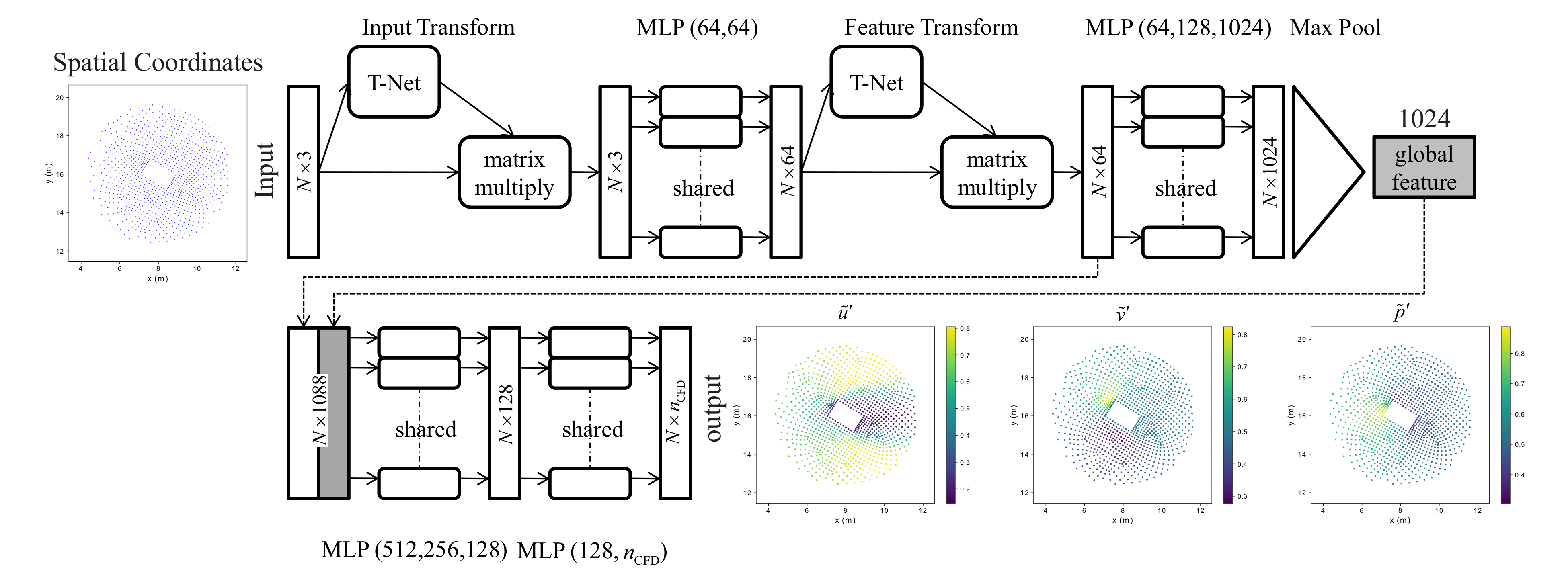
##### PointNet architecture #####
#We use the segmentation component of PointNet. One of the most important features of PointNet is its scalability.
#The variable `scaling` in the code allows users to make the network bigger or smaller to control its capacity.
#Please note that the `sigmoid` activation function is implemented in the last layer, since we normalize the output data in range of [0, 1].
#Additionally, we have removed T-Nets (Input Transforms and Feature Transforms) from the network implemented here. 
#However, please note that we had embedded T-Nets in the network in our [journal paper](https://aip.scitation.org/doi/figure/10.1063/5.0033376) (please see *Figure 5* of the journal paper).

scaling = 1.0 #reasonable choices for scaling: 4.0, 2.0, 1.0, 0.25, 0.125

def exp_dim(global_feature, num_points):
    return tf.tile(global_feature, [1, num_points, 1])

PointNet_input = Input(shape=(point_numbers, space_variable))
#Shared MLP (64,64)
branch1 = Convolution1D(int(64*scaling),1,input_shape=(point_numbers,space_variable), activation='relu')(PointNet_input)
branch1 = BatchNormalization()(branch1)
branch1 = Convolution1D(int(64*scaling),1,input_shape=(point_numbers,space_variable), activation='relu')(branch1)
branch1 = BatchNormalization()(branch1)
Local_Feature = branch1
#Shared MLP (64,128,1024)
branch1 = Convolution1D(int(64*scaling),1,activation='relu')(branch1)
branch1 = BatchNormalization()(branch1)
branch1 = Convolution1D(int(128*scaling),1,activation='relu')(branch1)
branch1 = BatchNormalization()(branch1)
branch1 = Convolution1D(int(1024*scaling),1,activation='relu')(branch1)
branch1 = BatchNormalization()(branch1)
#Max function
Global_Feature = MaxPooling1D(pool_size=int(point_numbers*scaling))(branch1)
Global_Feature = Lambda(exp_dim, arguments={'num_points':point_numbers})(Global_Feature)
branch2 = concatenate([Local_Feature, Global_Feature])
#Shared MLP (512,256,128)
branch2 = Convolution1D(int(512*scaling),1,activation='relu')(branch2)
branch2 = BatchNormalization()(branch2)
branch2 = Convolution1D(int(256*scaling),1,activation='relu')(branch2)
branch2 = BatchNormalization()(branch2)
branch2 = Convolution1D(int(128*scaling),1,activation='relu')(branch2)
branch2 = BatchNormalization()(branch2)
#Shared MLP (128, cfd_variable)
branch2 = Convolution1D(int(128*scaling),1,activation='relu')(branch2)
branch2 = BatchNormalization()(branch2)
PointNet_output = Convolution1D(cfd_variable,1,activation='sigmoid')(branch2) #Please note that we use the sigmoid activation function in the last layer.

##### Defining and compiling the model #####
#We use the `Adam` optimizer. Please note to the choice of `learning_rate` and `decaying_rate`. 
#The network is also sensitive to the choice of `epsilon` and it has to be set to a non-zero value.
#We use the `mean_squared_error` as the loss function (please see *Eq. 15* of the [journal paper](https://aip.scitation.org/doi/full/10.1063/5.0033376)).
#Please note that for your specific application, you need to tune the `learning_rate` and `decaying_rate`. 

learning_rate = 0.0005
decaying_rate = 0.0
model = Model(inputs=PointNet_input,outputs=PointNet_output)
model.compile(optimizers.Adam(lr=learning_rate, beta_1=0.9, beta_2=0.999, epsilon=0.000001, decay=decaying_rate)
                   , loss='mean_squared_error', metrics=['mean_squared_error'])

##### Training PointNet #####
#Please be careful about the choice of batch size (`batch`) and number of epochs (`epoch_number`).
#At the beginning, you might observe an increase in the validation loss, but please do not worry, it will eventually decrease.
#Please note that this section might take approximately 20 hours to be completed (if you are running the code on Google Colab). So, please be patient. 
#Alternatively, you can run this section on your cluster computing.

batch = 32
epoch_number = 4000
results = model.fit(input_training,output_training,batch_size=batch,epochs=epoch_number,shuffle=True,verbose=1, validation_split=0.0, validation_data=(input_validation, output_validation))

##### Plotting training history #####
#Trace of loss values over the training and validation set can be seen by plotting the history of training.

plt.plot(results.history['loss'])
plt.plot(results.history['val_loss'])
plt.yscale('log')
plt.ylabel('Loss')
plt.xlabel('Epoch')
plt.legend(['Training', 'Validation'], loc='upper left')
plt.savefig('Loss_History.png',dpi=300)
#plt.savefig('Loss_History.eps') #You can use this line for saving figures in EPS format  
plt.clf()
#plt.show()

##### Error analysis #####
#We can perform various error analyses. For example, here we are interested in the normalized root mean square error (RMSE).
#We compute the normalized root mean square error (pointwise) of the predicted velocity and pressure fields over each geometry of the test set, and then we take an average over all these domains. 
#We normalize the velocity error by the free stream velocity, which is 1 m/s. Moreover, we normalized the pressure error by the dynamic pressure (without the factor of 0.5) at the free stream.

average_RMSE_u = 0
average_RMSE_v = 0
average_RMSE_p = 0

test_set_number = test_idx.size
sample_point_cloud = zeros([1,point_numbers,space_variable],dtype='f')
truth_point_cloud = zeros([point_numbers,cfd_variable],dtype='f')

for s in range(test_set_number):
    for j in range(point_numbers):
        for i in range(space_variable):
            sample_point_cloud[0][j][i] = input_test[s][j][i]

    prediction = model.predict(sample_point_cloud, batch_size=None, verbose=0)
    
    #Unnormalized
    prediction[0,:,0] = prediction[0,:,0]*(u_max - u_min) + u_min 
    prediction[0,:,1] = prediction[0,:,1]*(v_max - v_min) + v_min
    prediction[0,:,2] = prediction[0,:,2]*(p_max - p_min) + p_min 

    output_test[s,:,0] = output_test[s,:,0]*(u_max - u_min) + u_min 
    output_test[s,:,1] = output_test[s,:,1]*(v_max - v_min) + v_min
    output_test[s,:,2] = output_test[s,:,2]*(p_max - p_min) + p_min

    average_RMSE_u += np.sqrt(np.sum(np.square(prediction[0,:,0]-output_test[s,:,0])))/point_numbers
    average_RMSE_v += np.sqrt(np.sum(np.square(prediction[0,:,1]-output_test[s,:,1])))/point_numbers
    average_RMSE_p += np.sqrt(np.sum(np.square(prediction[0,:,2]-output_test[s,:,2])))/point_numbers
    
average_RMSE_u = average_RMSE_u/test_set_number
average_RMSE_v = average_RMSE_v/test_set_number
average_RMSE_p = average_RMSE_p/test_set_number

print('Average normalized RMSE of the x-velocity component (u) over goemtries of the test set:')
print(average_RMSE_u)
print('Average normalized RMSE of the y-velocity component (v) over goemtries of the test set:')
print(average_RMSE_v)
print('Average normalized RMSE of the pressure (p) over goemtries of the test set:')
print(average_RMSE_p)

##### Visualizing the results #####
#For example, let us plot the velocity and pressure fields predicted by the network as well as absolute pointwise error distribution over these fields for one of the geometries of the test set.

s=0 #s can change from "0" to "test_set_number - 1"

for j in range(point_numbers):
    for i in range(space_variable):
        sample_point_cloud[0][j][i] = input_test[s][j][i]

prediction = model.predict(sample_point_cloud, batch_size=None, verbose=0)
    
#Unnormalized
prediction[0,:,0] = prediction[0,:,0]*(u_max - u_min) + u_min 
prediction[0,:,1] = prediction[0,:,1]*(v_max - v_min) + v_min
prediction[0,:,2] = prediction[0,:,2]*(p_max - p_min) + p_min 

#Please note that we have already unnormalized the 'output_test' in Sect. Error analysis.

plotSolution(sample_point_cloud[0,:,0],sample_point_cloud[0,:,1],prediction[0,:,0],'velocity prediction','velocity prediction (u)')
plotSolution(sample_point_cloud[0,:,0],sample_point_cloud[0,:,1],output_test[s,:,0],'velocity ground truth','velocity ground truth (u)')
plotSolution(sample_point_cloud[0,:,0],sample_point_cloud[0,:,1],np.absolute(output_test[s,:,0]-prediction[0,:,0]),'u_point_wise_error','absolute point-wise error of velocity (u) m/s')

plotSolution(sample_point_cloud[0,:,0],sample_point_cloud[0,:,1],prediction[0,:,1],'v_prediction','velocity prediction (v) m/s')
plotSolution(sample_point_cloud[0,:,0],sample_point_cloud[0,:,1],output_test[s,:,1],'v_ground_truth','velocity ground truth (v) m/s')
plotSolution(sample_point_cloud[0,:,0],sample_point_cloud[0,:,1],np.absolute(output_test[s,:,1]-prediction[0,:,1]),'v_point_wise_error','absolute point-wise error of velocity (v) m/s')

plotSolution(sample_point_cloud[0,:,0],sample_point_cloud[0,:,1],prediction[0,:,2],'p_prediction','pressure prediction (p) Pa')
plotSolution(sample_point_cloud[0,:,0],sample_point_cloud[0,:,1],output_test[s,:,2],'p_ground_truth','pressure ground truth (p) Pa')
plotSolution(sample_point_cloud[0,:,0],sample_point_cloud[0,:,1],np.absolute(output_test[s,:,2]-prediction[0,:,2]),'p_point_wise_error','absolute point-wise error of pressure (p) Pa')

#Questions?
#If you have any questions or need assistance,
#please do not hesitate to contact Ali Kashefi (kashefi@stanford.edu) or Davis Rempe (drempe@stanford.edu) via email.