Yolov8-源码解析-六-

Yolov8 源码解析（六）

comments: true
description: Master hyperparameter tuning for Ultralytics YOLO to optimize model performance with our comprehensive guide. Elevate your machine learning models today!.
keywords: Ultralytics YOLO, hyperparameter tuning, machine learning, model optimization, genetic algorithms, learning rate, batch size, epochs

Ultralytics YOLO Hyperparameter Tuning Guide

Introduction

Hyperparameter tuning is not just a one-time set-up but an iterative process aimed at optimizing the machine learning model's performance metrics, such as accuracy, precision, and recall. In the context of Ultralytics YOLO, these hyperparameters could range from learning rate to architectural details, such as the number of layers or types of activation functions used.

What are Hyperparameters?

Hyperparameters are high-level, structural settings for the algorithm. They are set prior to the training phase and remain constant during it. Here are some commonly tuned hyperparameters in Ultralytics YOLO:

Learning Rate lr0: Determines the step size at each iteration while moving towards a minimum in the loss function.
Batch Size batch: Number of images processed simultaneously in a forward pass.
Number of Epochs epochs: An epoch is one complete forward and backward pass of all the training examples.
Architecture Specifics: Such as channel counts, number of layers, types of activation functions, etc.

Hyperparameter Tuning Visual

For a full list of augmentation hyperparameters used in YOLOv8 please refer to the configurations page.

Genetic Evolution and Mutation

Ultralytics YOLO uses genetic algorithms to optimize hyperparameters. Genetic algorithms are inspired by the mechanism of natural selection and genetics.

Mutation: In the context of Ultralytics YOLO, mutation helps in locally searching the hyperparameter space by applying small, random changes to existing hyperparameters, producing new candidates for evaluation.
Crossover: Although crossover is a popular genetic algorithm technique, it is not currently used in Ultralytics YOLO for hyperparameter tuning. The focus is mainly on mutation for generating new hyperparameter sets.

Preparing for Hyperparameter Tuning

Before you begin the tuning process, it's important to:

Identify the Metrics: Determine the metrics you will use to evaluate the model's performance. This could be AP50, F1-score, or others.
Set the Tuning Budget: Define how much computational resources you're willing to allocate. Hyperparameter tuning can be computationally intensive.

Steps Involved

Initialize Hyperparameters

Start with a reasonable set of initial hyperparameters. This could either be the default hyperparameters set by Ultralytics YOLO or something based on your domain knowledge or previous experiments.

Mutate Hyperparameters

Use the _mutate method to produce a new set of hyperparameters based on the existing set.

Train Model

Training is performed using the mutated set of hyperparameters. The training performance is then assessed.

Evaluate Model

Use metrics like AP50, F1-score, or custom metrics to evaluate the model's performance.

Log Results

It's crucial to log both the performance metrics and the corresponding hyperparameters for future reference.

Repeat

The process is repeated until either the set number of iterations is reached or the performance metric is satisfactory.

Usage Example

Here's how to use the model.tune() method to utilize the Tuner class for hyperparameter tuning of YOLOv8n on COCO8 for 30 epochs with an AdamW optimizer and skipping plotting, checkpointing and validation other than on final epoch for faster Tuning.

!!! Example

=== "Python"

    ```py
    from ultralytics import YOLO

    # Initialize the YOLO model
    model = YOLO("yolov8n.pt")

    # Tune hyperparameters on COCO8 for 30 epochs
    model.tune(data="coco8.yaml", epochs=30, iterations=300, optimizer="AdamW", plots=False, save=False, val=False)
    ```

Results

After you've successfully completed the hyperparameter tuning process, you will obtain several files and directories that encapsulate the results of the tuning. The following describes each:

File Structure

Here's what the directory structure of the results will look like. Training directories like train1/ contain individual tuning iterations, i.e. one model trained with one set of hyperparameters. The tune/ directory contains tuning results from all the individual model trainings:

runs/
└── detect/
    ├── train1/
    ├── train2/
    ├── ...
    └── tune/
        ├── best_hyperparameters.yaml
        ├── best_fitness.png
        ├── tune_results.csv
        ├── tune_scatter_plots.png
        └── weights/
            ├── last.pt
            └── best.pt

File Descriptions

best_hyperparameters.yaml

This YAML file contains the best-performing hyperparameters found during the tuning process. You can use this file to initialize future trainings with these optimized settings.

Format: YAML
Usage: Hyperparameter results

Example:

# 558/900 iterations complete ✅ (45536.81s)
# Results saved to /usr/src/ultralytics/runs/detect/tune
# Best fitness=0.64297 observed at iteration 498
# Best fitness metrics are {'metrics/precision(B)': 0.87247, 'metrics/recall(B)': 0.71387, 'metrics/mAP50(B)': 0.79106, 'metrics/mAP50-95(B)': 0.62651, 'val/box_loss': 2.79884, 'val/cls_loss': 2.72386, 'val/dfl_loss': 0.68503, 'fitness': 0.64297}
# Best fitness model is /usr/src/ultralytics/runs/detect/train498
# Best fitness hyperparameters are printed below.

lr0: 0.00269
lrf: 0.00288
momentum: 0.73375
weight_decay: 0.00015
warmup_epochs: 1.22935
warmup_momentum: 0.1525
box: 18.27875
cls: 1.32899
dfl: 0.56016
hsv_h: 0.01148
hsv_s: 0.53554
hsv_v: 0.13636
degrees: 0.0
translate: 0.12431
scale: 0.07643
shear: 0.0
perspective: 0.0
flipud: 0.0
fliplr: 0.08631
mosaic: 0.42551
mixup: 0.0
copy_paste: 0.0

best_fitness.png

This is a plot displaying fitness (typically a performance metric like AP50) against the number of iterations. It helps you visualize how well the genetic algorithm performed over time.

Format: PNG
Usage: Performance visualization

Hyperparameter Tuning Fitness vs Iteration

tune_results.csv

A CSV file containing detailed results of each iteration during the tuning. Each row in the file represents one iteration, and it includes metrics like fitness score, precision, recall, as well as the hyperparameters used.

Format: CSV
Usage: Per-iteration results tracking.

Example:

  fitness,lr0,lrf,momentum,weight_decay,warmup_epochs,warmup_momentum,box,cls,dfl,hsv_h,hsv_s,hsv_v,degrees,translate,scale,shear,perspective,flipud,fliplr,mosaic,mixup,copy_paste
  0.05021,0.01,0.01,0.937,0.0005,3.0,0.8,7.5,0.5,1.5,0.015,0.7,0.4,0.0,0.1,0.5,0.0,0.0,0.0,0.5,1.0,0.0,0.0
  0.07217,0.01003,0.00967,0.93897,0.00049,2.79757,0.81075,7.5,0.50746,1.44826,0.01503,0.72948,0.40658,0.0,0.0987,0.4922,0.0,0.0,0.0,0.49729,1.0,0.0,0.0
  0.06584,0.01003,0.00855,0.91009,0.00073,3.42176,0.95,8.64301,0.54594,1.72261,0.01503,0.59179,0.40658,0.0,0.0987,0.46955,0.0,0.0,0.0,0.49729,0.80187,0.0,0.0

tune_scatter_plots.png

This file contains scatter plots generated from tune_results.csv, helping you visualize relationships between different hyperparameters and performance metrics. Note that hyperparameters initialized to 0 will not be tuned, such as degrees and shear below.

Format: PNG
Usage: Exploratory data analysis

Hyperparameter Tuning Scatter Plots

weights/

This directory contains the saved PyTorch models for the last and the best iterations during the hyperparameter tuning process.

last.pt: The last.pt are the weights from the last epoch of training.
best.pt: The best.pt weights for the iteration that achieved the best fitness score.

Using these results, you can make more informed decisions for your future model trainings and analyses. Feel free to consult these artifacts to understand how well your model performed and how you might improve it further.

Conclusion

The hyperparameter tuning process in Ultralytics YOLO is simplified yet powerful, thanks to its genetic algorithm-based approach focused on mutation. Following the steps outlined in this guide will assist you in systematically tuning your model to achieve better performance.

FAQ

How do I optimize the learning rate for Ultralytics YOLO during hyperparameter tuning?

To optimize the learning rate for Ultralytics YOLO, start by setting an initial learning rate using the lr0 parameter. Common values range from 0.001 to 0.01. During the hyperparameter tuning process, this value will be mutated to find the optimal setting. You can utilize the model.tune() method to automate this process. For example:

!!! Example

=== "Python"

    ```py
    from ultralytics import YOLO

    # Initialize the YOLO model
    model = YOLO("yolov8n.pt")

    # Tune hyperparameters on COCO8 for 30 epochs
    model.tune(data="coco8.yaml", epochs=30, iterations=300, optimizer="AdamW", plots=False, save=False, val=False)
    ```

For more details, check the Ultralytics YOLO configuration page.

What are the benefits of using genetic algorithms for hyperparameter tuning in YOLOv8?

Genetic algorithms in Ultralytics YOLOv8 provide a robust method for exploring the hyperparameter space, leading to highly optimized model performance. Key benefits include:

Efficient Search: Genetic algorithms like mutation can quickly explore a large set of hyperparameters.
Avoiding Local Minima: By introducing randomness, they help in avoiding local minima, ensuring better global optimization.
Performance Metrics: They adapt based on performance metrics such as AP50 and F1-score.

To see how genetic algorithms can optimize hyperparameters, check out the hyperparameter evolution guide.

How long does the hyperparameter tuning process take for Ultralytics YOLO?

The time required for hyperparameter tuning with Ultralytics YOLO largely depends on several factors such as the size of the dataset, the complexity of the model architecture, the number of iterations, and the computational resources available. For instance, tuning YOLOv8n on a dataset like COCO8 for 30 epochs might take several hours to days, depending on the hardware.

To effectively manage tuning time, define a clear tuning budget beforehand (internal section link). This helps in balancing resource allocation and optimization goals.

What metrics should I use to evaluate model performance during hyperparameter tuning in YOLO?

When evaluating model performance during hyperparameter tuning in YOLO, you can use several key metrics:

AP50: The average precision at IoU threshold of 0.50.
F1-Score: The harmonic mean of precision and recall.
Precision and Recall: Individual metrics indicating the model's accuracy in identifying true positives versus false positives and false negatives.

These metrics help you understand different aspects of your model's performance. Refer to the Ultralytics YOLO performance metrics guide for a comprehensive overview.

Can I use Ultralytics HUB for hyperparameter tuning of YOLO models?

Yes, you can use Ultralytics HUB for hyperparameter tuning of YOLO models. The HUB offers a no-code platform to easily upload datasets, train models, and perform hyperparameter tuning efficiently. It provides real-time tracking and visualization of tuning progress and results.

Explore more about using Ultralytics HUB for hyperparameter tuning in the Ultralytics HUB Cloud Training documentation.

comments: true
description: Master YOLO with Ultralytics tutorials covering training, deployment and optimization. Find solutions, improve metrics, and deploy with ease!.
keywords: Ultralytics, YOLO, tutorials, guides, object detection, deep learning, PyTorch, training, deployment, optimization, computer vision

Comprehensive Tutorials to Ultralytics YOLO

Welcome to the Ultralytics' YOLO 🚀 Guides! Our comprehensive tutorials cover various aspects of the YOLO object detection model, ranging from training and prediction to deployment. Built on PyTorch, YOLO stands out for its exceptional speed and accuracy in real-time object detection tasks.

Whether you're a beginner or an expert in deep learning, our tutorials offer valuable insights into the implementation and optimization of YOLO for your computer vision projects. Let's dive in!

Watch: Ultralytics YOLOv8 Guides Overview

Guides

Here's a compilation of in-depth guides to help you master different aspects of Ultralytics YOLO.

YOLO Common Issues ⭐ RECOMMENDED: Practical solutions and troubleshooting tips to the most frequently encountered issues when working with Ultralytics YOLO models.
YOLO Performance Metrics ⭐ ESSENTIAL: Understand the key metrics like mAP, IoU, and F1 score used to evaluate the performance of your YOLO models. Includes practical examples and tips on how to improve detection accuracy and speed.
Model Deployment Options: Overview of YOLO model deployment formats like ONNX, OpenVINO, and TensorRT, with pros and cons for each to inform your deployment strategy.
K-Fold Cross Validation 🚀 NEW: Learn how to improve model generalization using K-Fold cross-validation technique.
Hyperparameter Tuning 🚀 NEW: Discover how to optimize your YOLO models by fine-tuning hyperparameters using the Tuner class and genetic evolution algorithms.
SAHI Tiled Inference 🚀 NEW: Comprehensive guide on leveraging SAHI's sliced inference capabilities with YOLOv8 for object detection in high-resolution images.
AzureML Quickstart 🚀 NEW: Get up and running with Ultralytics YOLO models on Microsoft's Azure Machine Learning platform. Learn how to train, deploy, and scale your object detection projects in the cloud.
Conda Quickstart 🚀 NEW: Step-by-step guide to setting up a Conda environment for Ultralytics. Learn how to install and start using the Ultralytics package efficiently with Conda.
Docker Quickstart 🚀 NEW: Complete guide to setting up and using Ultralytics YOLO models with Docker. Learn how to install Docker, manage GPU support, and run YOLO models in isolated containers for consistent development and deployment.
Raspberry Pi 🚀 NEW: Quickstart tutorial to run YOLO models to the latest Raspberry Pi hardware.
NVIDIA Jetson 🚀 NEW: Quickstart guide for deploying YOLO models on NVIDIA Jetson devices.
DeepStream on NVIDIA Jetson 🚀 NEW: Quickstart guide for deploying YOLO models on NVIDIA Jetson devices using DeepStream and TensorRT.
Triton Inference Server Integration 🚀 NEW: Dive into the integration of Ultralytics YOLOv8 with NVIDIA's Triton Inference Server for scalable and efficient deep learning inference deployments.
YOLO Thread-Safe Inference 🚀 NEW: Guidelines for performing inference with YOLO models in a thread-safe manner. Learn the importance of thread safety and best practices to prevent race conditions and ensure consistent predictions.
Isolating Segmentation Objects 🚀 NEW: Step-by-step recipe and explanation on how to extract and/or isolate objects from images using Ultralytics Segmentation.
Edge TPU on Raspberry Pi: Google Edge TPU accelerates YOLO inference on Raspberry Pi.
View Inference Images in a Terminal: Use VSCode's integrated terminal to view inference results when using Remote Tunnel or SSH sessions.
OpenVINO Latency vs Throughput Modes - Learn latency and throughput optimization techniques for peak YOLO inference performance.
Steps of a Computer Vision Project 🚀 NEW: Learn about the key steps involved in a computer vision project, including defining goals, selecting models, preparing data, and evaluating results.
Defining A Computer Vision Project's Goals 🚀 NEW: Walk through how to effectively define clear and measurable goals for your computer vision project. Learn the importance of a well-defined problem statement and how it creates a roadmap for your project.
Data Collection and Annotation 🚀 NEW: Explore the tools, techniques, and best practices for collecting and annotating data to create high-quality inputs for your computer vision models.
Preprocessing Annotated Data 🚀 NEW: Learn about preprocessing and augmenting image data in computer vision projects using YOLOv8, including normalization, dataset augmentation, splitting, and exploratory data analysis (EDA).
Tips for Model Training 🚀 NEW: Explore tips on optimizing batch sizes, using mixed precision, applying pre-trained weights, and more to make training your computer vision model a breeze.
Insights on Model Evaluation and Fine-Tuning 🚀 NEW: Gain insights into the strategies and best practices for evaluating and fine-tuning your computer vision models. Learn about the iterative process of refining models to achieve optimal results.
A Guide on Model Testing 🚀 NEW: A thorough guide on testing your computer vision models in realistic settings. Learn how to verify accuracy, reliability, and performance in line with project goals.
Best Practices for Model Deployment 🚀 NEW: Walk through tips and best practices for efficiently deploying models in computer vision projects, with a focus on optimization, troubleshooting, and security.
Maintaining Your Computer Vision Model 🚀 NEW: Understand the key practices for monitoring, maintaining, and documenting computer vision models to guarantee accuracy, spot anomalies, and mitigate data drift.
ROS Quickstart 🚀 NEW: Learn how to integrate YOLO with the Robot Operating System (ROS) for real-time object detection in robotics applications, including Point Cloud and Depth images.

Contribute to Our Guides

We welcome contributions from the community! If you've mastered a particular aspect of Ultralytics YOLO that's not yet covered in our guides, we encourage you to share your expertise. Writing a guide is a great way to give back to the community and help us make our documentation more comprehensive and user-friendly.

To get started, please read our Contributing Guide for guidelines on how to open up a Pull Request (PR) 🛠️. We look forward to your contributions!

Let's work together to make the Ultralytics YOLO ecosystem more robust and versatile 🙏!

FAQ

How do I train a custom object detection model using Ultralytics YOLO?

Training a custom object detection model with Ultralytics YOLO is straightforward. Start by preparing your dataset in the correct format and installing the Ultralytics package. Use the following code to initiate training:

!!! Example

=== "Python"

    ```py
    from ultralytics import YOLO

    model = YOLO("yolov8s.pt")  # Load a pre-trained YOLO model
    model.train(data="path/to/dataset.yaml", epochs=50)  # Train on custom dataset
    ```

=== "CLI"

    ```py
    yolo task=detect mode=train model=yolov8s.pt data=path/to/dataset.yaml epochs=50
    ```

For detailed dataset formatting and additional options, refer to our Tips for Model Training guide.

What performance metrics should I use to evaluate my YOLO model?

Evaluating your YOLO model performance is crucial to understanding its efficacy. Key metrics include Mean Average Precision (mAP), Intersection over Union (IoU), and F1 score. These metrics help assess the accuracy and precision of object detection tasks. You can learn more about these metrics and how to improve your model in our YOLO Performance Metrics guide.

Why should I use Ultralytics HUB for my computer vision projects?

Ultralytics HUB is a no-code platform that simplifies managing, training, and deploying YOLO models. It supports seamless integration, real-time tracking, and cloud training, making it ideal for both beginners and professionals. Discover more about its features and how it can streamline your workflow with our Ultralytics HUB quickstart guide.

What are the common issues faced during YOLO model training, and how can I resolve them?

Common issues during YOLO model training include data formatting errors, model architecture mismatches, and insufficient training data. To address these, ensure your dataset is correctly formatted, check for compatible model versions, and augment your training data. For a comprehensive list of solutions, refer to our YOLO Common Issues guide.

How can I deploy my YOLO model for real-time object detection on edge devices?

Deploying YOLO models on edge devices like NVIDIA Jetson and Raspberry Pi requires converting the model to a compatible format such as TensorRT or TFLite. Follow our step-by-step guides for NVIDIA Jetson and Raspberry Pi deployments to get started with real-time object detection on edge hardware. These guides will walk you through installation, configuration, and performance optimization.

comments: true
description: Master instance segmentation and tracking with Ultralytics YOLOv8. Learn techniques for precise object identification and tracking.
keywords: instance segmentation, tracking, YOLOv8, Ultralytics, object detection, machine learning, computer vision, python

Instance Segmentation and Tracking using Ultralytics YOLOv8 🚀

What is Instance Segmentation?

Ultralytics YOLOv8 instance segmentation involves identifying and outlining individual objects in an image, providing a detailed understanding of spatial distribution. Unlike semantic segmentation, it uniquely labels and precisely delineates each object, crucial for tasks like object detection and medical imaging.

There are two types of instance segmentation tracking available in the Ultralytics package:

Instance Segmentation with Class Objects: Each class object is assigned a unique color for clear visual separation.
Instance Segmentation with Object Tracks: Every track is represented by a distinct color, facilitating easy identification and tracking.

Watch: Instance Segmentation with Object Tracking using Ultralytics YOLOv8

Samples

Instance Segmentation	Instance Segmentation + Object Tracking

Ultralytics Instance Segmentation 😍	Ultralytics Instance Segmentation with Object Tracking 🔥

!!! Example "Instance Segmentation and Tracking"

=== "Instance Segmentation"

    ```py
    import cv2

    from ultralytics import YOLO
    from ultralytics.utils.plotting import Annotator, colors

    model = YOLO("yolov8n-seg.pt")  # segmentation model
    names = model.model.names
    cap = cv2.VideoCapture("path/to/video/file.mp4")
    w, h, fps = (int(cap.get(x)) for x in (cv2.CAP_PROP_FRAME_WIDTH, cv2.CAP_PROP_FRAME_HEIGHT, cv2.CAP_PROP_FPS))

    out = cv2.VideoWriter("instance-segmentation.avi", cv2.VideoWriter_fourcc(*"MJPG"), fps, (w, h))

    while True:
        ret, im0 = cap.read()
        if not ret:
            print("Video frame is empty or video processing has been successfully completed.")
            break

        results = model.predict(im0)
        annotator = Annotator(im0, line_width=2)

        if results[0].masks is not None:
            clss = results[0].boxes.cls.cpu().tolist()
            masks = results[0].masks.xy
            for mask, cls in zip(masks, clss):
                color = colors(int(cls), True)
                txt_color = annotator.get_txt_color(color)
                annotator.seg_bbox(mask=mask, mask_color=color, label=names[int(cls)], txt_color=txt_color)

        out.write(im0)
        cv2.imshow("instance-segmentation", im0)

        if cv2.waitKey(1) & 0xFF == ord("q"):
            break

    out.release()
    cap.release()
    cv2.destroyAllWindows()
    ```

=== "Instance Segmentation with Object Tracking"

    ```py
    from collections import defaultdict

    import cv2

    from ultralytics import YOLO
    from ultralytics.utils.plotting import Annotator, colors

    track_history = defaultdict(lambda: [])

    model = YOLO("yolov8n-seg.pt")  # segmentation model
    cap = cv2.VideoCapture("path/to/video/file.mp4")
    w, h, fps = (int(cap.get(x)) for x in (cv2.CAP_PROP_FRAME_WIDTH, cv2.CAP_PROP_FRAME_HEIGHT, cv2.CAP_PROP_FPS))

    out = cv2.VideoWriter("instance-segmentation-object-tracking.avi", cv2.VideoWriter_fourcc(*"MJPG"), fps, (w, h))

    while True:
        ret, im0 = cap.read()
        if not ret:
            print("Video frame is empty or video processing has been successfully completed.")
            break

        annotator = Annotator(im0, line_width=2)

        results = model.track(im0, persist=True)

        if results[0].boxes.id is not None and results[0].masks is not None:
            masks = results[0].masks.xy
            track_ids = results[0].boxes.id.int().cpu().tolist()

            for mask, track_id in zip(masks, track_ids):
                color = colors(int(track_id), True)
                txt_color = annotator.get_txt_color(color)
                annotator.seg_bbox(mask=mask, mask_color=color, label=str(track_id), txt_color=txt_color)

        out.write(im0)
        cv2.imshow("instance-segmentation-object-tracking", im0)

        if cv2.waitKey(1) & 0xFF == ord("q"):
            break

    out.release()
    cap.release()
    cv2.destroyAllWindows()
    ```

`seg_bbox` Arguments

Name	Type	Default	Description
`mask`	`array`	`None`	Segmentation mask coordinates
`mask_color`	`RGB`	`(255, 0, 255)`	Mask color for every segmented box
`label`	`str`	`None`	Label for segmented object
`txt_color`	`RGB`	`None`	Label color for segmented and tracked object

Note

For any inquiries, feel free to post your questions in the Ultralytics Issue Section or the discussion section mentioned below.

FAQ

How do I perform instance segmentation using Ultralytics YOLOv8?

To perform instance segmentation using Ultralytics YOLOv8, initialize the YOLO model with a segmentation version of YOLOv8 and process video frames through it. Here's a simplified code example:

!!! Example

=== "Python"

    ```py
    import cv2

    from ultralytics import YOLO
    from ultralytics.utils.plotting import Annotator, colors

    model = YOLO("yolov8n-seg.pt")  # segmentation model
    cap = cv2.VideoCapture("path/to/video/file.mp4")
    w, h, fps = (int(cap.get(x)) for x in (cv2.CAP_PROP_FRAME_WIDTH, cv2.CAP_PROP_FRAME_HEIGHT, cv2.CAP_PROP_FPS))

    out = cv2.VideoWriter("instance-segmentation.avi", cv2.VideoWriter_fourcc(*"MJPG"), fps, (w, h))

    while True:
        ret, im0 = cap.read()
        if not ret:
            break

        results = model.predict(im0)
        annotator = Annotator(im0, line_width=2)

        if results[0].masks is not None:
            clss = results[0].boxes.cls.cpu().tolist()
            masks = results[0].masks.xy
            for mask, cls in zip(masks, clss):
                annotator.seg_bbox(mask=mask, mask_color=colors(int(cls), True), det_label=model.model.names[int(cls)])

        out.write(im0)
        cv2.imshow("instance-segmentation", im0)
        if cv2.waitKey(1) & 0xFF == ord("q"):
            break

    out.release()
    cap.release()
    cv2.destroyAllWindows()
    ```

Learn more about instance segmentation in the Ultralytics YOLOv8 guide.

What is the difference between instance segmentation and object tracking in Ultralytics YOLOv8?

Instance segmentation identifies and outlines individual objects within an image, giving each object a unique label and mask. Object tracking extends this by assigning consistent labels to objects across video frames, facilitating continuous tracking of the same objects over time. Learn more about the distinctions in the Ultralytics YOLOv8 documentation.

Why should I use Ultralytics YOLOv8 for instance segmentation and tracking over other models like Mask R-CNN or Faster R-CNN?

Ultralytics YOLOv8 offers real-time performance, superior accuracy, and ease of use compared to other models like Mask R-CNN or Faster R-CNN. YOLOv8 provides a seamless integration with Ultralytics HUB, allowing users to manage models, datasets, and training pipelines efficiently. Discover more about the benefits of YOLOv8 in the Ultralytics blog.

How can I implement object tracking using Ultralytics YOLOv8?

To implement object tracking, use the model.track method and ensure that each object's ID is consistently assigned across frames. Below is a simple example:

!!! Example

=== "Python"

    ```py
    from collections import defaultdict

    import cv2

    from ultralytics import YOLO
    from ultralytics.utils.plotting import Annotator, colors

    track_history = defaultdict(lambda: [])

    model = YOLO("yolov8n-seg.pt")  # segmentation model
    cap = cv2.VideoCapture("path/to/video/file.mp4")
    w, h, fps = (int(cap.get(x)) for x in (cv2.CAP_PROP_FRAME_WIDTH, cv2.CAP_PROP_FRAME_HEIGHT, cv2.CAP_PROP_FPS))

    out = cv2.VideoWriter("instance-segmentation-object-tracking.avi", cv2.VideoWriter_fourcc(*"MJPG"), fps, (w, h))

    while True:
        ret, im0 = cap.read()
        if not ret:
            break

        annotator = Annotator(im0, line_width=2)
        results = model.track(im0, persist=True)

        if results[0].boxes.id is not None and results[0].masks is not None:
            masks = results[0].masks.xy
            track_ids = results[0].boxes.id.int().cpu().tolist()

            for mask, track_id in zip(masks, track_ids):
                annotator.seg_bbox(mask=mask, mask_color=colors(track_id, True), track_label=str(track_id))

        out.write(im0)
        cv2.imshow("instance-segmentation-object-tracking", im0)
        if cv2.waitKey(1) & 0xFF == ord("q"):
            break

    out.release()
    cap.release()
    cv2.destroyAllWindows()
    ```

Find more in the Instance Segmentation and Tracking section.

Are there any datasets provided by Ultralytics suitable for training YOLOv8 models for instance segmentation and tracking?

Yes, Ultralytics offers several datasets suitable for training YOLOv8 models, including segmentation and tracking datasets. Dataset examples, structures, and instructions for use can be found in the Ultralytics Datasets documentation.

comments: true
description: Learn to extract isolated objects from inference results using Ultralytics Predict Mode. Step-by-step guide for segmentation object isolation.
keywords: Ultralytics, segmentation, object isolation, Predict Mode, YOLOv8, machine learning, object detection, binary mask, image processing

Isolating Segmentation Objects

After performing the Segment Task, it's sometimes desirable to extract the isolated objects from the inference results. This guide provides a generic recipe on how to accomplish this using the Ultralytics Predict Mode.

Example Isolated Object Segmentation

Recipe Walk Through

See the Ultralytics Quickstart Installation section for a quick walkthrough on installing the required libraries.

Load a model and run predict() method on a source.

from ultralytics import YOLO

# Load a model
model = YOLO("yolov8n-seg.pt")

# Run inference
results = model.predict()

!!! question "No Prediction Arguments?"

Without specifying a source, the example images from the library will be used:

```py
'ultralytics/assets/bus.jpg'
'ultralytics/assets/zidane.jpg'
```

This is helpful for rapid testing with the `predict()` method.

For additional information about Segmentation Models, visit the Segment Task page. To learn more about predict() method, see Predict Mode section of the Documentation.

Now iterate over the results and the contours. For workflows that want to save an image to file, the source image base-name and the detection class-label are retrieved for later use (optional).

from pathlib import Path

import numpy as np

# (2) Iterate detection results (helpful for multiple images)
for r in res:
    img = np.copy(r.orig_img)
    img_name = Path(r.path).stem  # source image base-name

    # Iterate each object contour (multiple detections)
    for ci, c in enumerate(r):
        # (1) Get detection class name
        label = c.names[c.boxes.cls.tolist().pop()]

To learn more about working with detection results, see Boxes Section for Predict Mode.
To learn more about predict() results see Working with Results for Predict Mode

??? info "For-Loop"

A single image will only iterate the first loop once. A single image with only a single detection will iterate each loop _only_ once.

Start with generating a binary mask from the source image and then draw a filled contour onto the mask. This will allow the object to be isolated from the other parts of the image. An example from bus.jpg for one of the detected person class objects is shown on the right.
```
import cv2

# Create binary mask
b_mask = np.zeros(img.shape[:2], np.uint8)

# (1) Extract contour result
contour = c.masks.xy.pop()
# (2) Changing the type
contour = contour.astype(np.int32)
# (3) Reshaping
contour = contour.reshape(-1, 1, 2)


# Draw contour onto mask
_ = cv2.drawContours(b_mask, [contour], -1, (255, 255, 255), cv2.FILLED)
```
1. For more info on c.masks.xy see Masks Section from Predict Mode.
2. Here the values are cast into np.int32 for compatibility with drawContours() function from OpenCV.
3. The OpenCV drawContours() function expects contours to have a shape of [N, 1, 2] expand section below for more details.
Expand to understand what is happening when defining the contour variable.
- c.masks.xy :: Provides the coordinates of the mask contour points in the format (x, y). For more details, refer to the Masks Section from Predict Mode.
- .pop() :: As masks.xy is a list containing a single element, this element is extracted using the pop() method.
- .astype(np.int32) :: Using masks.xy will return with a data type of float32, but this won't be compatible with the OpenCV drawContours() function, so this will change the data type to int32 for compatibility.
- .reshape(-1, 1, 2) :: Reformats the data into the required shape of [N, 1, 2] where N is the number of contour points, with each point represented by a single entry 1, and the entry is composed of 2 values. The -1 denotes that the number of values along this dimension is flexible.
Expand for an explanation of the drawContours() configuration.
- Encapsulating the contour variable within square brackets, [contour], was found to effectively generate the desired contour mask during testing.
- The value -1 specified for the drawContours() parameter instructs the function to draw all contours present in the image.
- The tuple (255, 255, 255) represents the color white, which is the desired color for drawing the contour in this binary mask.
- The addition of cv2.FILLED will color all pixels enclosed by the contour boundary the same, in this case, all enclosed pixels will be white.
- See OpenCV Documentation on drawContours() for more information.

Next there are 2 options for how to move forward with the image from this point and a subsequent option for each.

Object Isolation Options

!!! example ""

=== "Black Background Pixels"

    ```py
    # Create 3-channel mask
    mask3ch = cv2.cvtColor(b_mask, cv2.COLOR_GRAY2BGR)

    # Isolate object with binary mask
    isolated = cv2.bitwise_and(mask3ch, img)
    ```

    ??? question "How does this work?"

        - First, the binary mask is first converted from a single-channel image to a three-channel image. This conversion is necessary for the subsequent step where the mask and the original image are combined. Both images must have the same number of channels to be compatible with the blending operation.

        - The original image and the three-channel binary mask are merged using the OpenCV function `bitwise_and()`. This operation retains <u>only</u> pixel values that are greater than zero `(> 0)` from both images. Since the mask pixels are greater than zero `(> 0)` <u>only</u> within the contour region, the pixels remaining from the original image are those that overlap with the contour.

    ### Isolate with Black Pixels: Sub-options

    ??? info "Full-size Image"

        There are no additional steps required if keeping full size image.

        <figure markdown>
            ![Example Full size Isolated Object Image Black Background](https://github.com/ultralytics/ultralytics/assets/62214284/845c00d0-52a6-4b1e-8010-4ba73e011b99){ width=240 }
            <figcaption>Example full-size output</figcaption>
        </figure>

    ??? info "Cropped object Image"

        Additional steps required to crop image to only include object region.

        ![Example Crop Isolated Object Image Black Background](https://github.com/ultralytics/ultralytics/assets/62214284/103dbf90-c169-4f77-b791-76cdf09c6f22){ align="right" }
        ```py{ .py .annotate }
        # (1) Bounding box coordinates
        x1, y1, x2, y2 = c.boxes.xyxy.cpu().numpy().squeeze().astype(np.int32)
        # Crop image to object region
        iso_crop = isolated[y1:y2, x1:x2]
        ```

        1.  For more information on bounding box results, see [Boxes Section from Predict Mode](../modes/predict.md/#boxes)

        ??? question "What does this code do?"

            - The `c.boxes.xyxy.cpu().numpy()` call retrieves the bounding boxes as a NumPy array in the `xyxy` format, where `xmin`, `ymin`, `xmax`, and `ymax` represent the coordinates of the bounding box rectangle. See [Boxes Section from Predict Mode](../modes/predict.md/#boxes) for more details.

            - The `squeeze()` operation removes any unnecessary dimensions from the NumPy array, ensuring it has the expected shape.

            - Converting the coordinate values using `.astype(np.int32)` changes the box coordinates data type from `float32` to `int32`, making them compatible for image cropping using index slices.

            - Finally, the bounding box region is cropped from the image using index slicing. The bounds are defined by the `[ymin:ymax, xmin:xmax]` coordinates of the detection bounding box.

=== "Transparent Background Pixels"

    ```py
    # Isolate object with transparent background (when saved as PNG)
    isolated = np.dstack([img, b_mask])
    ```

    ??? question "How does this work?"

        - Using the NumPy `dstack()` function (array stacking along depth-axis) in conjunction with the binary mask generated, will create an image with four channels. This allows for all pixels outside of the object contour to be transparent when saving as a `PNG` file.

    ### Isolate with Transparent Pixels: Sub-options

    ??? info "Full-size Image"

        There are no additional steps required if keeping full size image.

        <figure markdown>
            ![Example Full size Isolated Object Image No Background](https://github.com/ultralytics/ultralytics/assets/62214284/b1043ee0-369a-4019-941a-9447a9771042){ width=240 }
            <figcaption>Example full-size output + transparent background</figcaption>
        </figure>

    ??? info "Cropped object Image"

        Additional steps required to crop image to only include object region.

        ![Example Crop Isolated Object Image No Background](https://github.com/ultralytics/ultralytics/assets/62214284/5910244f-d1e1-44af-af7f-6dea4c688da8){ align="right" }
        ```py{ .py .annotate }
        # (1) Bounding box coordinates
        x1, y1, x2, y2 = c.boxes.xyxy.cpu().numpy().squeeze().astype(np.int32)
        # Crop image to object region
        iso_crop = isolated[y1:y2, x1:x2]
        ```

        1.  For more information on bounding box results, see [Boxes Section from Predict Mode](../modes/predict.md/#boxes)

        ??? question "What does this code do?"

            - When using `c.boxes.xyxy.cpu().numpy()`, the bounding boxes are returned as a NumPy array, using the `xyxy` box coordinates format, which correspond to the points `xmin, ymin, xmax, ymax` for the bounding box (rectangle), see [Boxes Section from Predict Mode](../modes/predict.md/#boxes) for more information.

            - Adding `squeeze()` ensures that any extraneous dimensions are removed from the NumPy array.

            - Converting the coordinate values using `.astype(np.int32)` changes the box coordinates data type from `float32` to `int32` which will be compatible when cropping the image using index slices.

            - Finally the image region for the bounding box is cropped using index slicing, where the bounds are set using the `[ymin:ymax, xmin:xmax]` coordinates of the detection bounding box.

??? question "What if I want the cropped object including the background?"

This is a built in feature for the Ultralytics library. See the `save_crop` argument for  [Predict Mode Inference Arguments](../modes/predict.md/#inference-arguments) for details.

What to do next is entirely left to you as the developer. A basic example of one possible next step (saving the image to file for future use) is shown.

NOTE: this step is optional and can be skipped if not required for your specific use case.

??? example "Example Final Step"

```py
# Save isolated object to file
_ = cv2.imwrite(f"{img_name}_{label}-{ci}.png", iso_crop)
```

- In this example, the `img_name` is the base-name of the source image file, `label` is the detected class-name, and `ci` is the index of the object detection (in case of multiple instances with the same class name).

Full Example code

Here, all steps from the previous section are combined into a single block of code. For repeated use, it would be optimal to define a function to do some or all commands contained in the for-loops, but that is an exercise left to the reader.

from pathlib import Path

import cv2
import numpy as np

from ultralytics import YOLO

m = YOLO("yolov8n-seg.pt")  # (4)!
res = m.predict()  # (3)!

# Iterate detection results (5)
for r in res:
    img = np.copy(r.orig_img)
    img_name = Path(r.path).stem

    # Iterate each object contour (6)
    for ci, c in enumerate(r):
        label = c.names[c.boxes.cls.tolist().pop()]

        b_mask = np.zeros(img.shape[:2], np.uint8)

        # Create contour mask (1)
        contour = c.masks.xy.pop().astype(np.int32).reshape(-1, 1, 2)
        _ = cv2.drawContours(b_mask, [contour], -1, (255, 255, 255), cv2.FILLED)

        # Choose one:

        # OPTION-1: Isolate object with black background
        mask3ch = cv2.cvtColor(b_mask, cv2.COLOR_GRAY2BGR)
        isolated = cv2.bitwise_and(mask3ch, img)

        # OPTION-2: Isolate object with transparent background (when saved as PNG)
        isolated = np.dstack([img, b_mask])

        # OPTIONAL: detection crop (from either OPT1 or OPT2)
        x1, y1, x2, y2 = c.boxes.xyxy.cpu().numpy().squeeze().astype(np.int32)
        iso_crop = isolated[y1:y2, x1:x2]

        # TODO your actions go here (2)

The line populating contour is combined into a single line here, where it was split to multiple above.
{What goes here is up to you!}
See Predict Mode for additional information.
See Segment Task for more information.
Learn more about Working with Results
Learn more about Segmentation Mask Results

FAQ

How do I isolate objects using Ultralytics YOLOv8 for segmentation tasks?

To isolate objects using Ultralytics YOLOv8, follow these steps:

Load the model and run inference:

from ultralytics import YOLO

model = YOLO("yolov8n-seg.pt")
results = model.predict(source="path/to/your/image.jpg")

Generate a binary mask and draw contours:

import cv2
import numpy as np

img = np.copy(results[0].orig_img)
b_mask = np.zeros(img.shape[:2], np.uint8)
contour = results[0].masks.xy[0].astype(np.int32).reshape(-1, 1, 2)
cv2.drawContours(b_mask, [contour], -1, (255, 255, 255), cv2.FILLED)

Isolate the object using the binary mask:

mask3ch = cv2.cvtColor(b_mask, cv2.COLOR_GRAY2BGR)
isolated = cv2.bitwise_and(mask3ch, img)

Refer to the guide on Predict Mode and the Segment Task for more information.

What options are available for saving the isolated objects after segmentation?

Ultralytics YOLOv8 offers two main options for saving isolated objects:

With a Black Background:

mask3ch = cv2.cvtColor(b_mask, cv2.COLOR_GRAY2BGR)
isolated = cv2.bitwise_and(mask3ch, img)

With a Transparent Background:
```
isolated = np.dstack([img, b_mask])
```

For further details, visit the Predict Mode section.

How can I crop isolated objects to their bounding boxes using Ultralytics YOLOv8?

To crop isolated objects to their bounding boxes:

Retrieve bounding box coordinates:

x1, y1, x2, y2 = results[0].boxes.xyxy[0].cpu().numpy().astype(np.int32)

Crop the isolated image:
```
iso_crop = isolated[y1:y2, x1:x2]
```

Learn more about bounding box results in the Predict Mode documentation.

Why should I use Ultralytics YOLOv8 for object isolation in segmentation tasks?

Ultralytics YOLOv8 provides:

High-speed real-time object detection and segmentation.
Accurate bounding box and mask generation for precise object isolation.
Comprehensive documentation and easy-to-use API for efficient development.

Explore the benefits of using YOLO in the Segment Task documentation.

Can I save isolated objects including the background using Ultralytics YOLOv8?

Yes, this is a built-in feature in Ultralytics YOLOv8. Use the save_crop argument in the predict() method. For example:

results = model.predict(source="path/to/your/image.jpg", save_crop=True)

Read more about the save_crop argument in the Predict Mode Inference Arguments section.

comments: true
description: Learn to implement K-Fold Cross Validation for object detection datasets using Ultralytics YOLO. Improve your model's reliability and robustness.
keywords: Ultralytics, YOLO, K-Fold Cross Validation, object detection, sklearn, pandas, PyYaml, machine learning, dataset split

K-Fold Cross Validation with Ultralytics

Introduction

This comprehensive guide illustrates the implementation of K-Fold Cross Validation for object detection datasets within the Ultralytics ecosystem. We'll leverage the YOLO detection format and key Python libraries such as sklearn, pandas, and PyYaml to guide you through the necessary setup, the process of generating feature vectors, and the execution of a K-Fold dataset split.

K-Fold Cross Validation Overview

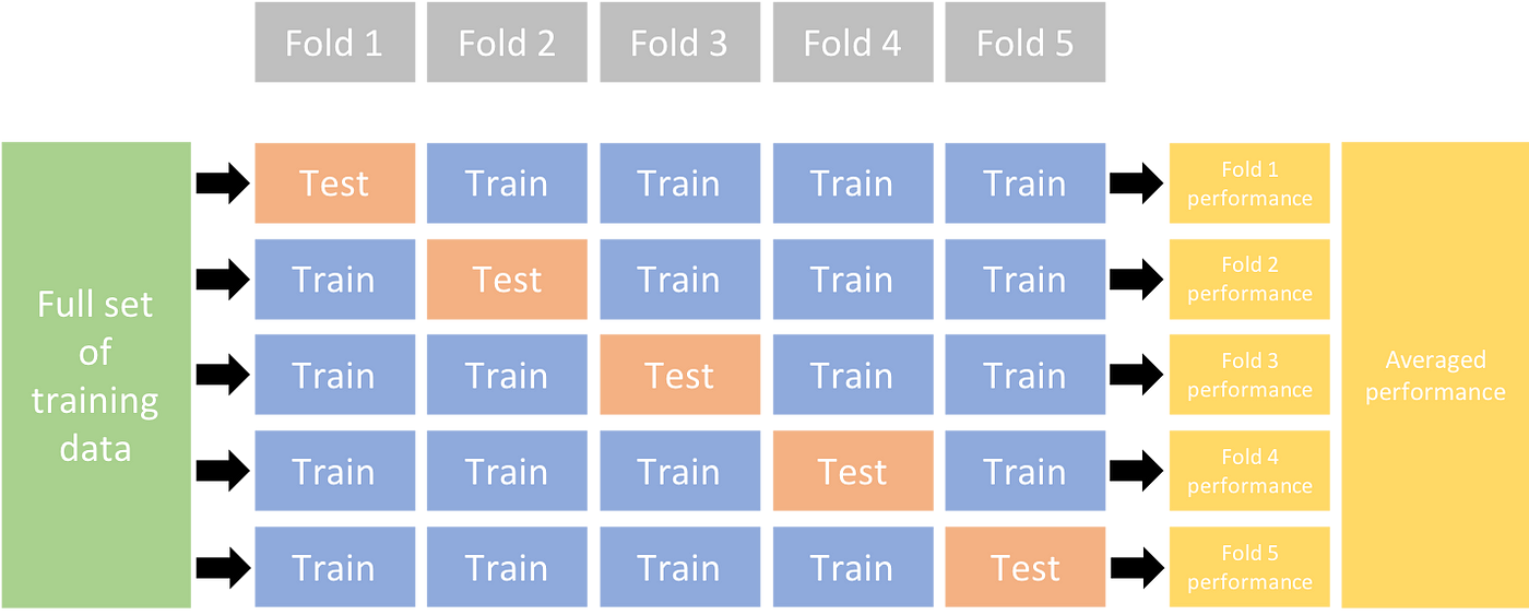
Whether your project involves the Fruit Detection dataset or a custom data source, this tutorial aims to help you comprehend and apply K-Fold Cross Validation to bolster the reliability and robustness of your machine learning models. While we're applying k=5 folds for this tutorial, keep in mind that the optimal number of folds can vary depending on your dataset and the specifics of your project.

Without further ado, let's dive in!

Setup

Your annotations should be in the YOLO detection format.
This guide assumes that annotation files are locally available.
For our demonstration, we use the Fruit Detection dataset.
- This dataset contains a total of 8479 images.
- It includes 6 class labels, each with its total instance counts listed below.

Class Label	Instance Count
Apple	7049
Grapes	7202
Pineapple	1613
Orange	15549
Banana	3536
Watermelon	1976

Necessary Python packages include:
- ultralytics
- sklearn
- pandas
- pyyaml
This tutorial operates with k=5 folds. However, you should determine the best number of folds for your specific dataset.

Initiate a new Python virtual environment (venv) for your project and activate it. Use pip (or your preferred package manager) to install:
- The Ultralytics library: pip install -U ultralytics. Alternatively, you can clone the official repo.
- Scikit-learn, pandas, and PyYAML: pip install -U scikit-learn pandas pyyaml.
Verify that your annotations are in the YOLO detection format.
- For this tutorial, all annotation files are found in the Fruit-Detection/labels directory.

Generating Feature Vectors for Object Detection Dataset

Start by creating a new example.py Python file for the steps below.

Proceed to retrieve all label files for your dataset.

from pathlib import Path

dataset_path = Path("./Fruit-detection")  # replace with 'path/to/dataset' for your custom data
labels = sorted(dataset_path.rglob("*labels/*.txt"))  # all data in 'labels'

Now, read the contents of the dataset YAML file and extract the indices of the class labels.

yaml_file = "path/to/data.yaml"  # your data YAML with data directories and names dictionary
with open(yaml_file, "r", encoding="utf8") as y:
    classes = yaml.safe_load(y)["names"]
cls_idx = sorted(classes.keys())

Initialize an empty pandas DataFrame.

import pandas as pd

indx = [l.stem for l in labels]  # uses base filename as ID (no extension)
labels_df = pd.DataFrame([], columns=cls_idx, index=indx)

Count the instances of each class-label present in the annotation files.

from collections import Counter

for label in labels:
    lbl_counter = Counter()

    with open(label, "r") as lf:
        lines = lf.readlines()

    for l in lines:
        # classes for YOLO label uses integer at first position of each line
        lbl_counter[int(l.split(" ")[0])] += 1

    labels_df.loc[label.stem] = lbl_counter

labels_df = labels_df.fillna(0.0)  # replace `nan` values with `0.0`

The following is a sample view of the populated DataFrame:

                                                       0    1    2    3    4    5
'0000a16e4b057580_jpg.rf.00ab48988370f64f5ca8ea4...'  0.0  0.0  0.0  0.0  0.0  7.0
'0000a16e4b057580_jpg.rf.7e6dce029fb67f01eb19aa7...'  0.0  0.0  0.0  0.0  0.0  7.0
'0000a16e4b057580_jpg.rf.bc4d31cdcbe229dd022957a...'  0.0  0.0  0.0  0.0  0.0  7.0
'00020ebf74c4881c_jpg.rf.508192a0a97aa6c4a3b6882...'  0.0  0.0  0.0  1.0  0.0  0.0
'00020ebf74c4881c_jpg.rf.5af192a2254c8ecc4188a25...'  0.0  0.0  0.0  1.0  0.0  0.0
 ...                                                  ...  ...  ...  ...  ...  ...
'ff4cd45896de38be_jpg.rf.c4b5e967ca10c7ced3b9e97...'  0.0  0.0  0.0  0.0  0.0  2.0
'ff4cd45896de38be_jpg.rf.ea4c1d37d2884b3e3cbce08...'  0.0  0.0  0.0  0.0  0.0  2.0
'ff5fd9c3c624b7dc_jpg.rf.bb519feaa36fc4bf630a033...'  1.0  0.0  0.0  0.0  0.0  0.0
'ff5fd9c3c624b7dc_jpg.rf.f0751c9c3aa4519ea3c9d6a...'  1.0  0.0  0.0  0.0  0.0  0.0
'fffe28b31f2a70d4_jpg.rf.7ea16bd637ba0711c53b540...'  0.0  6.0  0.0  0.0  0.0  0.0

The rows index the label files, each corresponding to an image in your dataset, and the columns correspond to your class-label indices. Each row represents a pseudo feature-vector, with the count of each class-label present in your dataset. This data structure enables the application of K-Fold Cross Validation to an object detection dataset.

K-Fold Dataset Split

Now we will use the KFold class from sklearn.model_selection to generate k splits of the dataset.
- Important:
  - Setting shuffle=True ensures a randomized distribution of classes in your splits.
  - By setting random_state=M where M is a chosen integer, you can obtain repeatable results.
```
from sklearn.model_selection import KFold

ksplit = 5
kf = KFold(n_splits=ksplit, shuffle=True, random_state=20)  # setting random_state for repeatable results

kfolds = list(kf.split(labels_df))
```

The dataset has now been split into k folds, each having a list of train and val indices. We will construct a DataFrame to display these results more clearly.

folds = [f"split_{n}" for n in range(1, ksplit + 1)]
folds_df = pd.DataFrame(index=indx, columns=folds)

for idx, (train, val) in enumerate(kfolds, start=1):
    folds_df[f"split_{idx}"].loc[labels_df.iloc[train].index] = "train"
    folds_df[f"split_{idx}"].loc[labels_df.iloc[val].index] = "val"

Now we will calculate the distribution of class labels for each fold as a ratio of the classes present in val to those present in train.

fold_lbl_distrb = pd.DataFrame(index=folds, columns=cls_idx)

for n, (train_indices, val_indices) in enumerate(kfolds, start=1):
    train_totals = labels_df.iloc[train_indices].sum()
    val_totals = labels_df.iloc[val_indices].sum()

    # To avoid division by zero, we add a small value (1E-7) to the denominator
    ratio = val_totals / (train_totals + 1e-7)
    fold_lbl_distrb.loc[f"split_{n}"] = ratio

The ideal scenario is for all class ratios to be reasonably similar for each split and across classes. This, however, will be subject to the specifics of your dataset.

Next, we create the directories and dataset YAML files for each split.

import datetime

supported_extensions = [".jpg", ".jpeg", ".png"]

# Initialize an empty list to store image file paths
images = []

# Loop through supported extensions and gather image files
for ext in supported_extensions:
    images.extend(sorted((dataset_path / "images").rglob(f"*{ext}")))

# Create the necessary directories and dataset YAML files (unchanged)
save_path = Path(dataset_path / f"{datetime.date.today().isoformat()}_{ksplit}-Fold_Cross-val")
save_path.mkdir(parents=True, exist_ok=True)
ds_yamls = []

for split in folds_df.columns:
    # Create directories
    split_dir = save_path / split
    split_dir.mkdir(parents=True, exist_ok=True)
    (split_dir / "train" / "images").mkdir(parents=True, exist_ok=True)
    (split_dir / "train" / "labels").mkdir(parents=True, exist_ok=True)
    (split_dir / "val" / "images").mkdir(parents=True, exist_ok=True)
    (split_dir / "val" / "labels").mkdir(parents=True, exist_ok=True)

    # Create dataset YAML files
    dataset_yaml = split_dir / f"{split}_dataset.yaml"
    ds_yamls.append(dataset_yaml)

    with open(dataset_yaml, "w") as ds_y:
        yaml.safe_dump(
            {
                "path": split_dir.as_posix(),
                "train": "train",
                "val": "val",
                "names": classes,
            },
            ds_y,
        )

Lastly, copy images and labels into the respective directory ('train' or 'val') for each split.

NOTE: The time required for this portion of the code will vary based on the size of your dataset and your system hardware.

import shutil

for image, label in zip(images, labels):
    for split, k_split in folds_df.loc[image.stem].items():
        # Destination directory
        img_to_path = save_path / split / k_split / "images"
        lbl_to_path = save_path / split / k_split / "labels"

        # Copy image and label files to new directory (SamefileError if file already exists)
        shutil.copy(image, img_to_path / image.name)
        shutil.copy(label, lbl_to_path / label.name)

Save Records (Optional)

Optionally, you can save the records of the K-Fold split and label distribution DataFrames as CSV files for future reference.

folds_df.to_csv(save_path / "kfold_datasplit.csv")
fold_lbl_distrb.to_csv(save_path / "kfold_label_distribution.csv")

Train YOLO using K-Fold Data Splits

First, load the YOLO model.

from ultralytics import YOLO

weights_path = "path/to/weights.pt"
model = YOLO(weights_path, task="detect")

Next, iterate over the dataset YAML files to run training. The results will be saved to a directory specified by the project and name arguments. By default, this directory is 'exp/runs#' where # is an integer index.

results = {}

# Define your additional arguments here
batch = 16
project = "kfold_demo"
epochs = 100

for k in range(ksplit):
    dataset_yaml = ds_yamls[k]
    model.train(data=dataset_yaml, epochs=epochs, batch=batch, project=project)  # include any train arguments
    results[k] = model.metrics  # save output metrics for further analysis

Conclusion

In this guide, we have explored the process of using K-Fold cross-validation for training the YOLO object detection model. We learned how to split our dataset into K partitions, ensuring a balanced class distribution across the different folds.

We also explored the procedure for creating report DataFrames to visualize the data splits and label distributions across these splits, providing us a clear insight into the structure of our training and validation sets.

Optionally, we saved our records for future reference, which could be particularly useful in large-scale projects or when troubleshooting model performance.

Finally, we implemented the actual model training using each split in a loop, saving our training results for further analysis and comparison.

This technique of K-Fold cross-validation is a robust way of making the most out of your available data, and it helps to ensure that your model performance is reliable and consistent across different data subsets. This results in a more generalizable and reliable model that is less likely to overfit to specific data patterns.

Remember that although we used YOLO in this guide, these steps are mostly transferable to other machine learning models. Understanding these steps allows you to apply cross-validation effectively in your own machine learning projects. Happy coding!

FAQ

What is K-Fold Cross Validation and why is it useful in object detection?

K-Fold Cross Validation is a technique where the dataset is divided into 'k' subsets (folds) to evaluate model performance more reliably. Each fold serves as both training and validation data. In the context of object detection, using K-Fold Cross Validation helps to ensure your Ultralytics YOLO model's performance is robust and generalizable across different data splits, enhancing its reliability. For detailed instructions on setting up K-Fold Cross Validation with Ultralytics YOLO, refer to K-Fold Cross Validation with Ultralytics.

How do I implement K-Fold Cross Validation using Ultralytics YOLO?

To implement K-Fold Cross Validation with Ultralytics YOLO, you need to follow these steps:

Verify annotations are in the YOLO detection format.
Use Python libraries like sklearn, pandas, and pyyaml.
Create feature vectors from your dataset.
Split your dataset using KFold from sklearn.model_selection.
Train the YOLO model on each split.

For a comprehensive guide, see the K-Fold Dataset Split section in our documentation.

Why should I use Ultralytics YOLO for object detection?

Ultralytics YOLO offers state-of-the-art, real-time object detection with high accuracy and efficiency. It's versatile, supporting multiple computer vision tasks such as detection, segmentation, and classification. Additionally, it integrates seamlessly with tools like Ultralytics HUB for no-code model training and deployment. For more details, explore the benefits and features on our Ultralytics YOLO page.

How can I ensure my annotations are in the correct format for Ultralytics YOLO?

Your annotations should follow the YOLO detection format. Each annotation file must list the object class, alongside its bounding box coordinates in the image. The YOLO format ensures streamlined and standardized data processing for training object detection models. For more information on proper annotation formatting, visit the YOLO detection format guide.

Can I use K-Fold Cross Validation with custom datasets other than Fruit Detection?

Yes, you can use K-Fold Cross Validation with any custom dataset as long as the annotations are in the YOLO detection format. Replace the dataset paths and class labels with those specific to your custom dataset. This flexibility ensures that any object detection project can benefit from robust model evaluation using K-Fold Cross Validation. For a practical example, review our Generating Feature Vectors section.

comments: true
description: Learn about YOLOv8's diverse deployment options to maximize your model's performance. Explore PyTorch, TensorRT, OpenVINO, TF Lite, and more!.
keywords: YOLOv8, deployment options, export formats, PyTorch, TensorRT, OpenVINO, TF Lite, machine learning, model deployment

Understanding YOLOv8's Deployment Options

Introduction

You've come a long way on your journey with YOLOv8. You've diligently collected data, meticulously annotated it, and put in the hours to train and rigorously evaluate your custom YOLOv8 model. Now, it's time to put your model to work for your specific application, use case, or project. But there's a critical decision that stands before you: how to export and deploy your model effectively.

This guide walks you through YOLOv8's deployment options and the essential factors to consider to choose the right option for your project.

How to Select the Right Deployment Option for Your YOLOv8 Model

When it's time to deploy your YOLOv8 model, selecting a suitable export format is very important. As outlined in the Ultralytics YOLOv8 Modes documentation, the model.export() function allows for converting your trained model into a variety of formats tailored to diverse environments and performance requirements.

The ideal format depends on your model's intended operational context, balancing speed, hardware constraints, and ease of integration. In the following section, we'll take a closer look at each export option, understanding when to choose each one.

YOLOv8's Deployment Options

Let's walk through the different YOLOv8 deployment options. For a detailed walkthrough of the export process, visit the Ultralytics documentation page on exporting.

PyTorch

PyTorch is an open-source machine learning library widely used for applications in deep learning and artificial intelligence. It provides a high level of flexibility and speed, which has made it a favorite among researchers and developers.

Performance Benchmarks: PyTorch is known for its ease of use and flexibility, which may result in a slight trade-off in raw performance when compared to other frameworks that are more specialized and optimized.
Compatibility and Integration: Offers excellent compatibility with various data science and machine learning libraries in Python.
Community Support and Ecosystem: One of the most vibrant communities, with extensive resources for learning and troubleshooting.
Case Studies: Commonly used in research prototypes, many academic papers reference models deployed in PyTorch.
Maintenance and Updates: Regular updates with active development and support for new features.
Security Considerations: Regular patches for security issues, but security is largely dependent on the overall environment it's deployed in.
Hardware Acceleration: Supports CUDA for GPU acceleration, essential for speeding up model training and inference.

TorchScript

TorchScript extends PyTorch's capabilities by allowing the exportation of models to be run in a C++ runtime environment. This makes it suitable for production environments where Python is unavailable.

Performance Benchmarks: Can offer improved performance over native PyTorch, especially in production environments.
Compatibility and Integration: Designed for seamless transition from PyTorch to C++ production environments, though some advanced features might not translate perfectly.
Community Support and Ecosystem: Benefits from PyTorch's large community but has a narrower scope of specialized developers.
Case Studies: Widely used in industry settings where Python's performance overhead is a bottleneck.
Maintenance and Updates: Maintained alongside PyTorch with consistent updates.
Security Considerations: Offers improved security by enabling the running of models in environments without full Python installations.
Hardware Acceleration: Inherits PyTorch's CUDA support, ensuring efficient GPU utilization.

ONNX

The Open Neural Network Exchange (ONNX) is a format that allows for model interoperability across different frameworks, which can be critical when deploying to various platforms.

Performance Benchmarks: ONNX models may experience a variable performance depending on the specific runtime they are deployed on.
Compatibility and Integration: High interoperability across multiple platforms and hardware due to its framework-agnostic nature.
Community Support and Ecosystem: Supported by many organizations, leading to a broad ecosystem and a variety of tools for optimization.
Case Studies: Frequently used to move models between different machine learning frameworks, demonstrating its flexibility.
Maintenance and Updates: As an open standard, ONNX is regularly updated to support new operations and models.
Security Considerations: As with any cross-platform tool, it's essential to ensure secure practices in the conversion and deployment pipeline.
Hardware Acceleration: With ONNX Runtime, models can leverage various hardware optimizations.

OpenVINO

OpenVINO is an Intel toolkit designed to facilitate the deployment of deep learning models across Intel hardware, enhancing performance and speed.

Performance Benchmarks: Specifically optimized for Intel CPUs, GPUs, and VPUs, offering significant performance boosts on compatible hardware.
Compatibility and Integration: Works best within the Intel ecosystem but also supports a range of other platforms.
Community Support and Ecosystem: Backed by Intel, with a solid user base especially in the computer vision domain.
Case Studies: Often utilized in IoT and edge computing scenarios where Intel hardware is prevalent.
Maintenance and Updates: Intel regularly updates OpenVINO to support the latest deep learning models and Intel hardware.
Security Considerations: Provides robust security features suitable for deployment in sensitive applications.
Hardware Acceleration: Tailored for acceleration on Intel hardware, leveraging dedicated instruction sets and hardware features.

For more details on deployment using OpenVINO, refer to the Ultralytics Integration documentation: Intel OpenVINO Export.

TensorRT

TensorRT is a high-performance deep learning inference optimizer and runtime from NVIDIA, ideal for applications needing speed and efficiency.

Performance Benchmarks: Delivers top-tier performance on NVIDIA GPUs with support for high-speed inference.
Compatibility and Integration: Best suited for NVIDIA hardware, with limited support outside this environment.
Community Support and Ecosystem: Strong support network through NVIDIA's developer forums and documentation.
Case Studies: Widely adopted in industries requiring real-time inference on video and image data.
Maintenance and Updates: NVIDIA maintains TensorRT with frequent updates to enhance performance and support new GPU architectures.
Security Considerations: Like many NVIDIA products, it has a strong emphasis on security, but specifics depend on the deployment environment.
Hardware Acceleration: Exclusively designed for NVIDIA GPUs, providing deep optimization and acceleration.

CoreML

CoreML is Apple's machine learning framework, optimized for on-device performance in the Apple ecosystem, including iOS, macOS, watchOS, and tvOS.

Performance Benchmarks: Optimized for on-device performance on Apple hardware with minimal battery usage.
Compatibility and Integration: Exclusively for Apple's ecosystem, providing a streamlined workflow for iOS and macOS applications.
Community Support and Ecosystem: Strong support from Apple and a dedicated developer community, with extensive documentation and tools.
Case Studies: Commonly used in applications that require on-device machine learning capabilities on Apple products.
Maintenance and Updates: Regularly updated by Apple to support the latest machine learning advancements and Apple hardware.
Security Considerations: Benefits from Apple's focus on user privacy and data security.
Hardware Acceleration: Takes full advantage of Apple's neural engine and GPU for accelerated machine learning tasks.

TF SavedModel

TF SavedModel is TensorFlow's format for saving and serving machine learning models, particularly suited for scalable server environments.

Performance Benchmarks: Offers scalable performance in server environments, especially when used with TensorFlow Serving.
Compatibility and Integration: Wide compatibility across TensorFlow's ecosystem, including cloud and enterprise server deployments.
Community Support and Ecosystem: Large community support due to TensorFlow's popularity, with a vast array of tools for deployment and optimization.
Case Studies: Extensively used in production environments for serving deep learning models at scale.
Maintenance and Updates: Supported by Google and the TensorFlow community, ensuring regular updates and new features.
Security Considerations: Deployment using TensorFlow Serving includes robust security features for enterprise-grade applications.
Hardware Acceleration: Supports various hardware accelerations through TensorFlow's backends.

TF GraphDef

TF GraphDef is a TensorFlow format that represents the model as a graph, which is beneficial for environments where a static computation graph is required.

Performance Benchmarks: Provides stable performance for static computation graphs, with a focus on consistency and reliability.
Compatibility and Integration: Easily integrates within TensorFlow's infrastructure but less flexible compared to SavedModel.
Community Support and Ecosystem: Good support from TensorFlow's ecosystem, with many resources available for optimizing static graphs.
Case Studies: Useful in scenarios where a static graph is necessary, such as in certain embedded systems.
Maintenance and Updates: Regular updates alongside TensorFlow's core updates.
Security Considerations: Ensures safe deployment with TensorFlow's established security practices.
Hardware Acceleration: Can utilize TensorFlow's hardware acceleration options, though not as flexible as SavedModel.

TF Lite

TF Lite is TensorFlow's solution for mobile and embedded device machine learning, providing a lightweight library for on-device inference.

Performance Benchmarks: Designed for speed and efficiency on mobile and embedded devices.
Compatibility and Integration: Can be used on a wide range of devices due to its lightweight nature.
Community Support and Ecosystem: Backed by Google, it has a robust community and a growing number of resources for developers.
Case Studies: Popular in mobile applications that require on-device inference with minimal footprint.
Maintenance and Updates: Regularly updated to include the latest features and optimizations for mobile devices.
Security Considerations: Provides a secure environment for running models on end-user devices.
Hardware Acceleration: Supports a variety of hardware acceleration options, including GPU and DSP.

TF Edge TPU

TF Edge TPU is designed for high-speed, efficient computing on Google's Edge TPU hardware, perfect for IoT devices requiring real-time processing.

Performance Benchmarks: Specifically optimized for high-speed, efficient computing on Google's Edge TPU hardware.
Compatibility and Integration: Works exclusively with TensorFlow Lite models on Edge TPU devices.
Community Support and Ecosystem: Growing support with resources provided by Google and third-party developers.
Case Studies: Used in IoT devices and applications that require real-time processing with low latency.
Maintenance and Updates: Continually improved upon to leverage the capabilities of new Edge TPU hardware releases.
Security Considerations: Integrates with Google's robust security for IoT and edge devices.
Hardware Acceleration: Custom-designed to take full advantage of Google Coral devices.

TF.js

TensorFlow.js (TF.js) is a library that brings machine learning capabilities directly to the browser, offering a new realm of possibilities for web developers and users alike. It allows for the integration of machine learning models in web applications without the need for back-end infrastructure.

Performance Benchmarks: Enables machine learning directly in the browser with reasonable performance, depending on the client device.
Compatibility and Integration: High compatibility with web technologies, allowing for easy integration into web applications.
Community Support and Ecosystem: Support from a community of web and Node.js developers, with a variety of tools for deploying ML models in browsers.
Case Studies: Ideal for interactive web applications that benefit from client-side machine learning without the need for server-side processing.
Maintenance and Updates: Maintained by the TensorFlow team with contributions from the open-source community.
Security Considerations: Runs within the browser's secure context, utilizing the security model of the web platform.
Hardware Acceleration: Performance can be enhanced with web-based APIs that access hardware acceleration like WebGL.

PaddlePaddle

PaddlePaddle is an open-source deep learning framework developed by Baidu. It is designed to be both efficient for researchers and easy to use for developers. It's particularly popular in China and offers specialized support for Chinese language processing.

Performance Benchmarks: Offers competitive performance with a focus on ease of use and scalability.
Compatibility and Integration: Well-integrated within Baidu's ecosystem and supports a wide range of applications.
Community Support and Ecosystem: While the community is smaller globally, it's rapidly growing, especially in China.
Case Studies: Commonly used in Chinese markets and by developers looking for alternatives to other major frameworks.
Maintenance and Updates: Regularly updated with a focus on serving Chinese language AI applications and services.
Security Considerations: Emphasizes data privacy and security, catering to Chinese data governance standards.
Hardware Acceleration: Supports various hardware accelerations, including Baidu's own Kunlun chips.

NCNN

NCNN is a high-performance neural network inference framework optimized for the mobile platform. It stands out for its lightweight nature and efficiency, making it particularly well-suited for mobile and embedded devices where resources are limited.

Performance Benchmarks: Highly optimized for mobile platforms, offering efficient inference on ARM-based devices.
Compatibility and Integration: Suitable for applications on mobile phones and embedded systems with ARM architecture.
Community Support and Ecosystem: Supported by a niche but active community focused on mobile and embedded ML applications.
Case Studies: Favoured for mobile applications where efficiency and speed are critical on Android and other ARM-based systems.
Maintenance and Updates: Continuously improved to maintain high performance on a range of ARM devices.
Security Considerations: Focuses on running locally on the device, leveraging the inherent security of on-device processing.
Hardware Acceleration: Tailored for ARM CPUs and GPUs, with specific optimizations for these architectures.

Comparative Analysis of YOLOv8 Deployment Options

The following table provides a snapshot of the various deployment options available for YOLOv8 models, helping you to assess which may best fit your project needs based on several critical criteria. For an in-depth look at each deployment option's format, please see the Ultralytics documentation page on export formats.

Deployment Option	Performance Benchmarks	Compatibility and Integration	Community Support and Ecosystem	Case Studies	Maintenance and Updates	Security Considerations	Hardware Acceleration
PyTorch	Good flexibility; may trade off raw performance	Excellent with Python libraries	Extensive resources and community	Research and prototypes	Regular, active development	Dependent on deployment environment	CUDA support for GPU acceleration
TorchScript	Better for production than PyTorch	Smooth transition from PyTorch to C++	Specialized but narrower than PyTorch	Industry where Python is a bottleneck	Consistent updates with PyTorch	Improved security without full Python	Inherits CUDA support from PyTorch
ONNX	Variable depending on runtime	High across different frameworks	Broad ecosystem, supported by many orgs	Flexibility across ML frameworks	Regular updates for new operations	Ensure secure conversion and deployment practices	Various hardware optimizations
OpenVINO	Optimized for Intel hardware	Best within Intel ecosystem	Solid in computer vision domain	IoT and edge with Intel hardware	Regular updates for Intel hardware	Robust features for sensitive applications	Tailored for Intel hardware
TensorRT	Top-tier on NVIDIA GPUs	Best for NVIDIA hardware	Strong network through NVIDIA	Real-time video and image inference	Frequent updates for new GPUs	Emphasis on security	Designed for NVIDIA GPUs
CoreML	Optimized for on-device Apple hardware	Exclusive to Apple ecosystem	Strong Apple and developer support	On-device ML on Apple products	Regular Apple updates	Focus on privacy and security	Apple neural engine and GPU
TF SavedModel	Scalable in server environments	Wide compatibility in TensorFlow ecosystem	Large support due to TensorFlow popularity	Serving models at scale	Regular updates by Google and community	Robust features for enterprise	Various hardware accelerations
TF GraphDef	Stable for static computation graphs	Integrates well with TensorFlow infrastructure	Resources for optimizing static graphs	Scenarios requiring static graphs	Updates alongside TensorFlow core	Established TensorFlow security practices	TensorFlow acceleration options
TF Lite	Speed and efficiency on mobile/embedded	Wide range of device support	Robust community, Google backed	Mobile applications with minimal footprint	Latest features for mobile	Secure environment on end-user devices	GPU and DSP among others
TF Edge TPU	Optimized for Google's Edge TPU hardware	Exclusive to Edge TPU devices	Growing with Google and third-party resources	IoT devices requiring real-time processing	Improvements for new Edge TPU hardware	Google's robust IoT security	Custom-designed for Google Coral
TF.js	Reasonable in-browser performance	High with web technologies	Web and Node.js developers support	Interactive web applications	TensorFlow team and community contributions	Web platform security model	Enhanced with WebGL and other APIs
PaddlePaddle	Competitive, easy to use and scalable	Baidu ecosystem, wide application support	Rapidly growing, especially in China	Chinese market and language processing	Focus on Chinese AI applications	Emphasizes data privacy and security	Including Baidu's Kunlun chips
NCNN	Optimized for mobile ARM-based devices	Mobile and embedded ARM systems	Niche but active mobile/embedded ML community	Android and ARM systems efficiency	High performance maintenance on ARM	On-device security advantages	ARM CPUs and GPUs optimizations

This comparative analysis gives you a high-level overview. For deployment, it's essential to consider the specific requirements and constraints of your project, and consult the detailed documentation and resources available for each option.

Community and Support

When you're getting started with YOLOv8, having a helpful community and support can make a significant impact. Here's how to connect with others who share your interests and get the assistance you need.

Engage with the Broader Community

GitHub Discussions: The YOLOv8 repository on GitHub has a "Discussions" section where you can ask questions, report issues, and suggest improvements.
Ultralytics Discord Server: Ultralytics has a Discord server where you can interact with other users and developers.

Official Documentation and Resources

Ultralytics YOLOv8 Docs: The official documentation provides a comprehensive overview of YOLOv8, along with guides on installation, usage, and troubleshooting.

These resources will help you tackle challenges and stay updated on the latest trends and best practices in the YOLOv8 community.

Conclusion

In this guide, we've explored the different deployment options for YOLOv8. We've also discussed the important factors to consider when making your choice. These options allow you to customize your model for various environments and performance requirements, making it suitable for real-world applications.

Don't forget that the YOLOv8 and Ultralytics community is a valuable source of help. Connect with other developers and experts to learn unique tips and solutions you might not find in regular documentation. Keep seeking knowledge, exploring new ideas, and sharing your experiences.

Happy deploying!

FAQ

What are the deployment options available for YOLOv8 on different hardware platforms?

Ultralytics YOLOv8 supports various deployment formats, each designed for specific environments and hardware platforms. Key formats include:

PyTorch for research and prototyping, with excellent Python integration.
TorchScript for production environments where Python is unavailable.
ONNX for cross-platform compatibility and hardware acceleration.
OpenVINO for optimized performance on Intel hardware.
TensorRT for high-speed inference on NVIDIA GPUs.

Each format has unique advantages. For a detailed walkthrough, see our export process documentation.

How do I improve the inference speed of my YOLOv8 model on an Intel CPU?

To enhance inference speed on Intel CPUs, you can deploy your YOLOv8 model using Intel's OpenVINO toolkit. OpenVINO offers significant performance boosts by optimizing models to leverage Intel hardware efficiently.

Convert your YOLOv8 model to the OpenVINO format using the model.export() function.
Follow the detailed setup guide in the Intel OpenVINO Export documentation.

For more insights, check out our blog post.

Can I deploy YOLOv8 models on mobile devices?

Yes, YOLOv8 models can be deployed on mobile devices using TensorFlow Lite (TF Lite) for both Android and iOS platforms. TF Lite is designed for mobile and embedded devices, providing efficient on-device inference.

!!! Example

=== "Python"

    ```py
    # Export command for TFLite format
    model.export(format="tflite")
    ```

=== "CLI"

    ```py
    # CLI command for TFLite export
    yolo export --format tflite
    ```

For more details on deploying models to mobile, refer to our TF Lite integration guide.

What factors should I consider when choosing a deployment format for my YOLOv8 model?

When choosing a deployment format for YOLOv8, consider the following factors:

Performance: Some formats like TensorRT provide exceptional speeds on NVIDIA GPUs, while OpenVINO is optimized for Intel hardware.
Compatibility: ONNX offers broad compatibility across different platforms.
Ease of Integration: Formats like CoreML or TF Lite are tailored for specific ecosystems like iOS and Android, respectively.
Community Support: Formats like PyTorch and TensorFlow have extensive community resources and support.

For a comparative analysis, refer to our export formats documentation.

How can I deploy YOLOv8 models in a web application?

To deploy YOLOv8 models in a web application, you can use TensorFlow.js (TF.js), which allows for running machine learning models directly in the browser. This approach eliminates the need for backend infrastructure and provides real-time performance.

Export the YOLOv8 model to the TF.js format.
Integrate the exported model into your web application.

For step-by-step instructions, refer to our guide on TensorFlow.js integration.

comments: true
description: Learn essential tips, insights, and best practices for deploying computer vision models with a focus on efficiency, optimization, troubleshooting, and maintaining security.
keywords: Model Deployment, Machine Learning Model Deployment, ML Model Deployment, AI Model Deployment, How to Deploy a Machine Learning Model, How to Deploy ML Models

Best Practices for Model Deployment

Introduction

Model deployment is the step in a computer vision project that brings a model from the development phase into a real-world application. There are various model deployment options: cloud deployment offers scalability and ease of access, edge deployment reduces latency by bringing the model closer to the data source, and local deployment ensures privacy and control. Choosing the right strategy depends on your application's needs, balancing speed, security, and scalability.

It's also important to follow best practices when deploying a model because deployment can significantly impact the effectiveness and reliability of the model's performance. In this guide, we'll focus on how to make sure that your model deployment is smooth, efficient, and secure.

Model Deployment Options

Often times, once a model is trained, evaluated, and tested, it needs to be converted into specific formats to be deployed effectively in various environments, such as cloud, edge, or local devices.

With respect to YOLOv8, you can export your model to different formats. For example, when you need to transfer your model between different frameworks, ONNX is an excellent tool and exporting to YOLOv8 to ONNX is easy. You can check out more options about integrating your model into different environments smoothly and effectively here.

Choosing a Deployment Environment

Choosing where to deploy your computer vision model depends on multiple factors. Different environments have unique benefits and challenges, so it's essential to pick the one that best fits your needs.

Cloud Deployment

Cloud deployment is great for applications that need to scale up quickly and handle large amounts of data. Platforms like AWS, Google Cloud, and Azure make it easy to manage your models from training to deployment. They offer services like AWS SageMaker, Google AI Platform, and Azure Machine Learning to help you throughout the process.

However, using the cloud can be expensive, especially with high data usage, and you might face latency issues if your users are far from the data centers. To manage costs and performance, it's important to optimize resource use and ensure compliance with data privacy rules.

Edge Deployment

Edge deployment works well for applications needing real-time responses and low latency, particularly in places with limited or no internet access. Deploying models on edge devices like smartphones or IoT gadgets ensures fast processing and keeps data local, which enhances privacy. Deploying on edge also saves bandwidth due to reduced data sent to the cloud.

However, edge devices often have limited processing power, so you'll need to optimize your models. Tools like TensorFlow Lite and NVIDIA Jetson can help. Despite the benefits, maintaining and updating many devices can be challenging.

Local Deployment

Local Deployment is best when data privacy is critical or when there's unreliable or no internet access. Running models on local servers or desktops gives you full control and keeps your data secure. It can also reduce latency if the server is near the user.

However, scaling locally can be tough, and maintenance can be time-consuming. Using tools like Docker for containerization and Kubernetes for management can help make local deployments more efficient. Regular updates and maintenance are necessary to keep everything running smoothly.

Model Optimization Techniques

Optimizing your computer vision model helps it runs efficiently, especially when deploying in environments with limited resources like edge devices. Here are some key techniques for optimizing your model.

Model Pruning

Pruning reduces the size of the model by removing weights that contribute little to the final output. It makes the model smaller and faster without significantly affecting accuracy. Pruning involves identifying and eliminating unnecessary parameters, resulting in a lighter model that requires less computational power. It is particularly useful for deploying models on devices with limited resources.

Model Pruning Overview

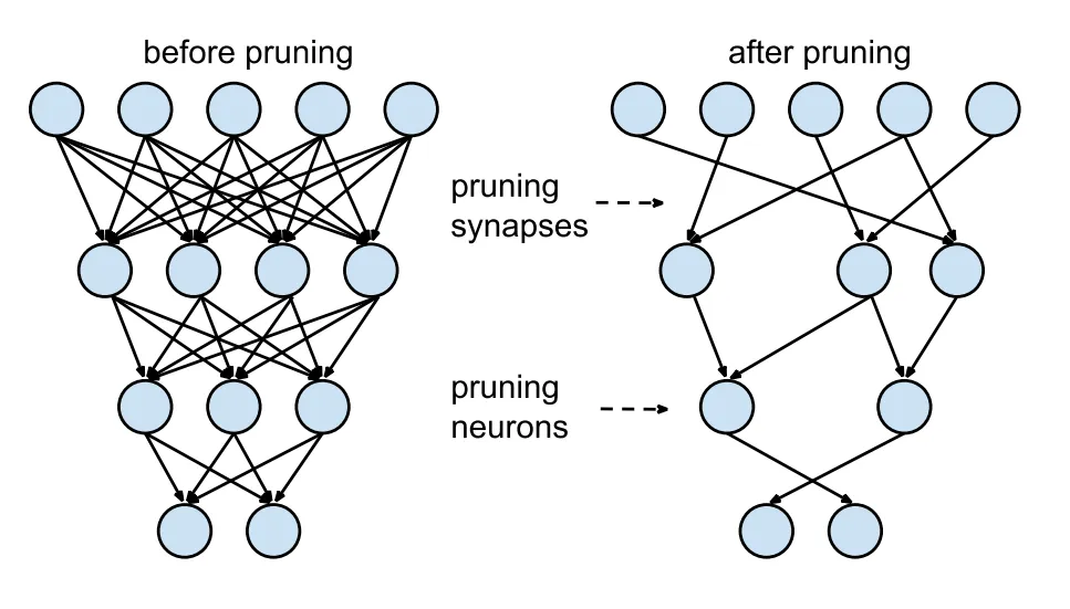
Model Quantization

Quantization converts the model's weights and activations from high precision (like 32-bit floats) to lower precision (like 8-bit integers). By reducing the model size, it speeds up inference. Quantization-aware training (QAT) is a method where the model is trained with quantization in mind, preserving accuracy better than post-training quantization. By handling quantization during the training phase, the model learns to adjust to lower precision, maintaining performance while reducing computational demands.

Model Quantization Overview

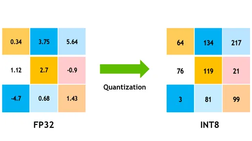
Knowledge Distillation

Knowledge distillation involves training a smaller, simpler model (the student) to mimic the outputs of a larger, more complex model (the teacher). The student model learns to approximate the teacher's predictions, resulting in a compact model that retains much of the teacher's accuracy. This technique is beneficial for creating efficient models suitable for deployment on edge devices with constrained resources.

Knowledge Distillation Overview

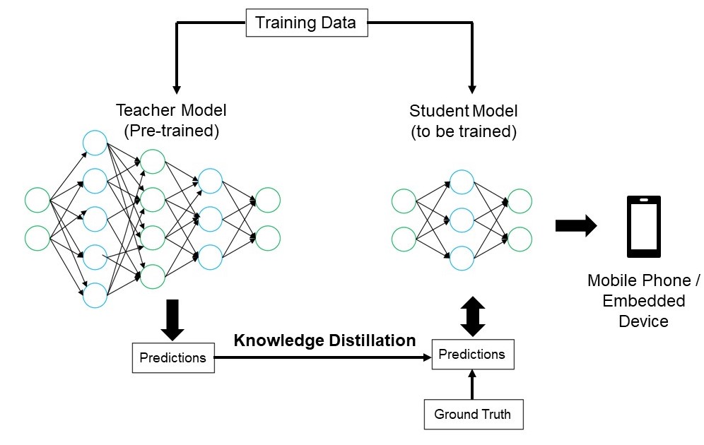
Troubleshooting Deployment Issues

You may face challenges while deploying your computer vision models, but understanding common problems and solutions can make the process smoother. Here are some general troubleshooting tips and best practices to help you navigate deployment issues.

Your Model is Less Accurate After Deployment

Experiencing a drop in your model's accuracy after deployment can be frustrating. This issue can stem from various factors. Here are some steps to help you identify and resolve the problem:

Check Data Consistency: Check that the data your model is processing post-deployment is consistent with the data it was trained on. Differences in data distribution, quality, or format can significantly impact performance.
Validate Preprocessing Steps: Verify that all preprocessing steps applied during training are also applied consistently during deployment. This includes resizing images, normalizing pixel values, and other data transformations.
Evaluate the Model's Environment: Ensure that the hardware and software configurations used during deployment match those used during training. Differences in libraries, versions, and hardware capabilities can introduce discrepancies.
Monitor Model Inference: Log inputs and outputs at various stages of the inference pipeline to detect any anomalies. It can help identify issues like data corruption or improper handling of model outputs.
Review Model Export and Conversion: Re-export the model and make sure that the conversion process maintains the integrity of the model weights and architecture.
Test with a Controlled Dataset: Deploy the model in a test environment with a dataset you control and compare the results with the training phase. You can identify if the issue is with the deployment environment or the data.

When deploying YOLOv8, several factors can affect model accuracy. Converting models to formats like TensorRT involves optimizations such as weight quantization and layer fusion, which can cause minor precision losses. Using FP16 (half-precision) instead of FP32 (full-precision) can speed up inference but may introduce numerical precision errors. Also, hardware constraints, like those on the Jetson Nano, with lower CUDA core counts and reduced memory bandwidth, can impact performance.

Inferences Are Taking Longer Than You Expected

When deploying machine learning models, it's important that they run efficiently. If inferences are taking longer than expected, it can affect the user experience and the effectiveness of your application. Here are some steps to help you identify and resolve the problem:

Implement Warm-Up Runs: Initial runs often include setup overhead, which can skew latency measurements. Perform a few warm-up inferences before measuring latency. Excluding these initial runs provides a more accurate measurement of the model's performance.
Optimize the Inference Engine: Double-check that the inference engine is fully optimized for your specific GPU architecture. Use the latest drivers and software versions tailored to your hardware to ensure maximum performance and compatibility.
Use Asynchronous Processing: Asynchronous processing can help manage workloads more efficiently. Use asynchronous processing techniques to handle multiple inferences concurrently, which can help distribute the load and reduce wait times.
Profile the Inference Pipeline: Identifying bottlenecks in the inference pipeline can help pinpoint the source of delays. Use profiling tools to analyze each step of the inference process, identifying and addressing any stages that cause significant delays, such as inefficient layers or data transfer issues.
Use Appropriate Precision: Using higher precision than necessary can slow down inference times. Experiment with using lower precision, such as FP16 (half-precision), instead of FP32 (full-precision). While FP16 can reduce inference time, also keep in mind that it can impact model accuracy.

If you are facing this issue while deploying YOLOv8, consider that YOLOv8 offers various model sizes, such as YOLOv8n (nano) for devices with lower memory capacity and YOLOv8x (extra-large) for more powerful GPUs. Choosing the right model variant for your hardware can help balance memory usage and processing time.

Also keep in mind that the size of the input images directly impacts memory usage and processing time. Lower resolutions reduce memory usage and speed up inference, while higher resolutions improve accuracy but require more memory and processing power.

Security Considerations in Model Deployment

Another important aspect of deployment is security. The security of your deployed models is critical to protect sensitive data and intellectual property. Here are some best practices you can follow related to secure model deployment.

Secure Data Transmission

Making sure data sent between clients and servers is secure is very important to prevent it from being intercepted or accessed by unauthorized parties. You can use encryption protocols like TLS (Transport Layer Security) to encrypt data while it's being transmitted. Even if someone intercepts the data, they won't be able to read it. You can also use end-to-end encryption that protects the data all the way from the source to the destination, so no one in between can access it.

Access Controls

It's essential to control who can access your model and its data to prevent unauthorized use. Use strong authentication methods to verify the identity of users or systems trying to access the model, and consider adding extra security with multi-factor authentication (MFA). Set up role-based access control (RBAC) to assign permissions based on user roles so that people only have access to what they need. Keep detailed audit logs to track all access and changes to the model and its data, and regularly review these logs to spot any suspicious activity.

Model Obfuscation

Protecting your model from being reverse-engineered or misuse can be done through model obfuscation. It involves encrypting model parameters, such as weights and biases in neural networks, to make it difficult for unauthorized individuals to understand or alter the model. You can also obfuscate the model's architecture by renaming layers and parameters or adding dummy layers, making it harder for attackers to reverse-engineer it. You can also serve the model in a secure environment, like a secure enclave or using a trusted execution environment (TEE), can provide an extra layer of protection during inference.

Being part of a community of computer vision enthusiasts can help you solve problems and learn faster. Here are some ways to connect, get help, and share ideas.

Community Resources

GitHub Issues: Explore the YOLOv8 GitHub repository and use the Issues tab to ask questions, report bugs, and suggest new features. The community and maintainers are very active and ready to help.
Ultralytics Discord Server: Join the Ultralytics Discord server to chat with other users and developers, get support, and share your experiences.

Official Documentation

Ultralytics YOLOv8 Documentation: Visit the official YOLOv8 documentation for detailed guides and helpful tips on various computer vision projects.

Using these resources will help you solve challenges and stay up-to-date with the latest trends and practices in the computer vision community.

Conclusion and Next Steps

We walked through some best practices to follow when deploying computer vision models. By securing data, controlling access, and obfuscating model details, you can protect sensitive information while keeping your models running smoothly. We also discussed how to address common issues like reduced accuracy and slow inferences using strategies such as warm-up runs, optimizing engines, asynchronous processing, profiling pipelines, and choosing the right precision.

After deploying your model, the next step would be monitoring, maintaining, and documenting your application. Regular monitoring helps catch and fix issues quickly, maintenance keeps your models up-to-date and functional, and good documentation tracks all changes and updates. These steps will help you achieve the goals of your computer vision project.

FAQ

What are the best practices for deploying a machine learning model using Ultralytics YOLOv8?

Deploying a machine learning model, particularly with Ultralytics YOLOv8, involves several best practices to ensure efficiency and reliability. First, choose the deployment environment that suits your needs—cloud, edge, or local. Optimize your model through techniques like pruning, quantization, and knowledge distillation for efficient deployment in resource-constrained environments. Lastly, ensure data consistency and preprocessing steps align with the training phase to maintain performance. You can also refer to model deployment options for more detailed guidelines.

How can I troubleshoot common deployment issues with Ultralytics YOLOv8 models?

Troubleshooting deployment issues can be broken down into a few key steps. If your model's accuracy drops after deployment, check for data consistency, validate preprocessing steps, and ensure the hardware/software environment matches what you used during training. For slow inference times, perform warm-up runs, optimize your inference engine, use asynchronous processing, and profile your inference pipeline. Refer to troubleshooting deployment issues for a detailed guide on these best practices.

How does Ultralytics YOLOv8 optimization enhance model performance on edge devices?

Optimizing Ultralytics YOLOv8 models for edge devices involves using techniques like pruning to reduce the model size, quantization to convert weights to lower precision, and knowledge distillation to train smaller models that mimic larger ones. These techniques ensure the model runs efficiently on devices with limited computational power. Tools like TensorFlow Lite and NVIDIA Jetson are particularly useful for these optimizations. Learn more about these techniques in our section on model optimization.

What are the security considerations for deploying machine learning models with Ultralytics YOLOv8?

Security is paramount when deploying machine learning models. Ensure secure data transmission using encryption protocols like TLS. Implement robust access controls, including strong authentication and role-based access control (RBAC). Model obfuscation techniques, such as encrypting model parameters and serving models in a secure environment like a trusted execution environment (TEE), offer additional protection. For detailed practices, refer to security considerations.

How do I choose the right deployment environment for my Ultralytics YOLOv8 model?

Selecting the optimal deployment environment for your Ultralytics YOLOv8 model depends on your application's specific needs. Cloud deployment offers scalability and ease of access, making it ideal for applications with high data volumes. Edge deployment is best for low-latency applications requiring real-time responses, using tools like TensorFlow Lite. Local deployment suits scenarios needing stringent data privacy and control. For a comprehensive overview of each environment, check out our section on choosing a deployment environment.

comments: true
description: Explore the most effective ways to assess and refine YOLOv8 models for better performance. Learn about evaluation metrics, fine-tuning processes, and how to customize your model for specific needs.
keywords: Model Evaluation, Machine Learning Model Evaluation, Fine Tuning Machine Learning, Fine Tune Model, Evaluating Models, Model Fine Tuning, How to Fine Tune a Model

Insights on Model Evaluation and Fine-Tuning

Introduction

Once you've trained your computer vision model, evaluating and refining it to perform optimally is essential. Just training your model isn't enough. You need to make sure that your model is accurate, efficient, and fulfills the objective of your computer vision project. By evaluating and fine-tuning your model, you can identify weaknesses, improve its accuracy, and boost overall performance.

In this guide, we'll share insights on model evaluation and fine-tuning that'll make this step of a computer vision project more approachable. We'll discuss how to understand evaluation metrics and implement fine-tuning techniques, giving you the knowledge to elevate your model's capabilities.

Evaluating Model Performance Using Metrics

Evaluating how well a model performs helps us understand how effectively it works. Various metrics are used to measure performance. These performance metrics provide clear, numerical insights that can guide improvements toward making sure the model meets its intended goals. Let's take a closer look at a few key metrics.

Confidence Score

The confidence score represents the model's certainty that a detected object belongs to a particular class. It ranges from 0 to 1, with higher scores indicating greater confidence. The confidence score helps filter predictions; only detections with confidence scores above a specified threshold are considered valid.

Quick Tip: When running inferences, if you aren't seeing any predictions and you've checked everything else, try lowering the confidence score. Sometimes, the threshold is too high, causing the model to ignore valid predictions. Lowering the score allows the model to consider more possibilities. This might not meet your project goals, but it's a good way to see what the model can do and decide how to fine-tune it.

Intersection over Union

Intersection over Union (IoU) is a metric in object detection that measures how well the predicted bounding box overlaps with the ground truth bounding box. IoU values range from 0 to 1, where one stands for a perfect match. IoU is essential because it measures how closely the predicted boundaries match the actual object boundaries.

Intersection over Union Overview

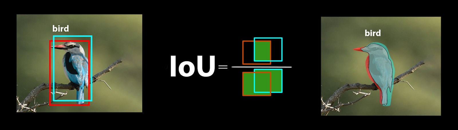
Mean Average Precision

Mean Average Precision (mAP) is a way to measure how well an object detection model performs. It looks at the precision of detecting each object class, averages these scores, and gives an overall number that shows how accurately the model can identify and classify objects.

Let's focus on two specific mAP metrics:

mAP@.5: Measures the average precision at a single IoU (Intersection over Union) threshold of 0.5. This metric checks if the model can correctly find objects with a looser accuracy requirement. It focuses on whether the object is roughly in the right place, not needing perfect placement. It helps see if the model is generally good at spotting objects.
mAP@.5:.95: Averages the mAP values calculated at multiple IoU thresholds, from 0.5 to 0.95 in 0.05 increments. This metric is more detailed and strict. It gives a fuller picture of how accurately the model can find objects at different levels of strictness and is especially useful for applications that need precise object detection.

Other mAP metrics include mAP@0.75, which uses a stricter IoU threshold of 0.75, and mAP@small, medium, and large, which evaluate precision across objects of different sizes.

Mean Average Precision Overview

Evaluating YOLOv8 Model Performance

With respect to YOLOv8, you can use the validation mode to evaluate the model. Also, be sure to take a look at our guide that goes in-depth into YOLOv8 performance metrics and how they can be interpreted.

Common Community Questions

When evaluating your YOLOv8 model, you might run into a few hiccups. Based on common community questions, here are some tips to help you get the most out of your YOLOv8 model:

Handling Variable Image Sizes

Evaluating your YOLOv8 model with images of different sizes can help you understand its performance on diverse datasets. Using the rect=true validation parameter, YOLOv8 adjusts the network's stride for each batch based on the image sizes, allowing the model to handle rectangular images without forcing them to a single size.

The imgsz validation parameter sets the maximum dimension for image resizing, which is 640 by default. You can adjust this based on your dataset's maximum dimensions and the GPU memory available. Even with imgsz set, rect=true lets the model manage varying image sizes effectively by dynamically adjusting the stride.

Accessing YOLOv8 Metrics

If you want to get a deeper understanding of your YOLOv8 model's performance, you can easily access specific evaluation metrics with a few lines of Python code. The code snippet below will let you load your model, run an evaluation, and print out various metrics that show how well your model is doing.

!!! Example "Usage"

=== "Python"

    ```py
    from ultralytics import YOLO

    # Load the model
    model = YOLO("yolov8n.pt")

    # Run the evaluation
    results = model.val(data="coco8.yaml")

    # Print specific metrics
    print("Class indices with average precision:", results.ap_class_index)
    print("Average precision for all classes:", results.box.all_ap)
    print("Average precision:", results.box.ap)
    print("Average precision at IoU=0.50:", results.box.ap50)
    print("Class indices for average precision:", results.box.ap_class_index)
    print("Class-specific results:", results.box.class_result)
    print("F1 score:", results.box.f1)
    print("F1 score curve:", results.box.f1_curve)
    print("Overall fitness score:", results.box.fitness)
    print("Mean average precision:", results.box.map)
    print("Mean average precision at IoU=0.50:", results.box.map50)
    print("Mean average precision at IoU=0.75:", results.box.map75)
    print("Mean average precision for different IoU thresholds:", results.box.maps)
    print("Mean results for different metrics:", results.box.mean_results)
    print("Mean precision:", results.box.mp)
    print("Mean recall:", results.box.mr)
    print("Precision:", results.box.p)
    print("Precision curve:", results.box.p_curve)
    print("Precision values:", results.box.prec_values)
    print("Specific precision metrics:", results.box.px)
    print("Recall:", results.box.r)
    print("Recall curve:", results.box.r_curve)
    ```

The results object also includes speed metrics like preprocess time, inference time, loss, and postprocess time. By analyzing these metrics, you can fine-tune and optimize your YOLOv8 model for better performance, making it more effective for your specific use case.

How Does Fine-Tuning Work?

Fine-tuning involves taking a pre-trained model and adjusting its parameters to improve performance on a specific task or dataset. The process, also known as model retraining, allows the model to better understand and predict outcomes for the specific data it will encounter in real-world applications. You can retrain your model based on your model evaluation to achieve optimal results.

Tips for Fine-Tuning Your Model

Fine-tuning a model means paying close attention to several vital parameters and techniques to achieve optimal performance. Here are some essential tips to guide you through the process.

Starting With a Higher Learning Rate

Usually, during the initial training epochs, the learning rate starts low and gradually increases to stabilize the training process. However, since your model has already learned some features from the previous dataset, starting with a higher learning rate right away can be more beneficial.

When evaluating your YOLOv8 model, you can set the warmup_epochs validation parameter to warmup_epochs=0 to prevent the learning rate from starting too high. By following this process, the training will continue from the provided weights, adjusting to the nuances of your new data.

Image Tiling for Small Objects

Image tiling can improve detection accuracy for small objects. By dividing larger images into smaller segments, such as splitting 1280x1280 images into multiple 640x640 segments, you maintain the original resolution, and the model can learn from high-resolution fragments. When using YOLOv8, make sure to adjust your labels for these new segments correctly.

Engage with the Community

Sharing your ideas and questions with other computer vision enthusiasts can inspire creative solutions to roadblocks in your projects. Here are some excellent ways to learn, troubleshoot, and connect.

Finding Help and Support

GitHub Issues: Explore the YOLOv8 GitHub repository and use the Issues tab to ask questions, report bugs, and suggest features. The community and maintainers are available to assist with any issues you encounter.
Ultralytics Discord Server: Join the Ultralytics Discord server to connect with other users and developers, get support, share knowledge, and brainstorm ideas.

Official Documentation

Ultralytics YOLOv8 Documentation: Check out the official YOLOv8 documentation for comprehensive guides and valuable insights on various computer vision tasks and projects.

Final Thoughts

Evaluating and fine-tuning your computer vision model are important steps for successful model deployment. These steps help make sure that your model is accurate, efficient, and suited to your overall application. The key to training the best model possible is continuous experimentation and learning. Don't hesitate to tweak parameters, try new techniques, and explore different datasets. Keep experimenting and pushing the boundaries of what's possible!

FAQ

What are the key metrics for evaluating YOLOv8 model performance?

To evaluate YOLOv8 model performance, important metrics include Confidence Score, Intersection over Union (IoU), and Mean Average Precision (mAP). Confidence Score measures the model's certainty for each detected object class. IoU evaluates how well the predicted bounding box overlaps with the ground truth. Mean Average Precision (mAP) aggregates precision scores across classes, with mAP@.5 and mAP@.5:.95 being two common types for varying IoU thresholds. Learn more about these metrics in our YOLOv8 performance metrics guide.

How can I fine-tune a pre-trained YOLOv8 model for my specific dataset?

Fine-tuning a pre-trained YOLOv8 model involves adjusting its parameters to improve performance on a specific task or dataset. Start by evaluating your model using metrics, then set a higher initial learning rate by adjusting the warmup_epochs parameter to 0 for immediate stability. Use parameters like rect=true for handling varied image sizes effectively. For more detailed guidance, refer to our section on fine-tuning YOLOv8 models.

How can I handle variable image sizes when evaluating my YOLOv8 model?

To handle variable image sizes during evaluation, use the rect=true parameter in YOLOv8, which adjusts the network's stride for each batch based on image sizes. The imgsz parameter sets the maximum dimension for image resizing, defaulting to 640. Adjust imgsz to suit your dataset and GPU memory. For more details, visit our section on handling variable image sizes.

What practical steps can I take to improve mean average precision for my YOLOv8 model?

Improving mean average precision (mAP) for a YOLOv8 model involves several steps:

Tuning Hyperparameters: Experiment with different learning rates, batch sizes, and image augmentations.
Data Augmentation: Use techniques like Mosaic and MixUp to create diverse training samples.
Image Tiling: Split larger images into smaller tiles to improve detection accuracy for small objects.
Refer to our detailed guide on model fine-tuning for specific strategies.

How do I access YOLOv8 model evaluation metrics in Python?

You can access YOLOv8 model evaluation metrics using Python with the following steps:

!!! Example "Usage"

=== "Python"

    ```py
    from ultralytics import YOLO

    # Load the model
    model = YOLO("yolov8n.pt")

    # Run the evaluation
    results = model.val(data="coco8.yaml")

    # Print specific metrics
    print("Class indices with average precision:", results.ap_class_index)
    print("Average precision for all classes:", results.box.all_ap)
    print("Mean average precision at IoU=0.50:", results.box.map50)
    print("Mean recall:", results.box.mr)
    ```

Analyzing these metrics helps fine-tune and optimize your YOLOv8 model. For a deeper dive, check out our guide on YOLOv8 metrics.

posted @ 2024-09-05 11:58 绝不原创的飞龙阅读(1) 评论(0) 编辑收藏举报

会员力量，点亮园子希望

刷新页面返回顶部

龙哥盟

掠夺·扩张·投机·博弈

Yolov8-源码解析-六-

Yolov8 源码解析（六）

Ultralytics YOLO Hyperparameter Tuning Guide

Introduction

What are Hyperparameters?

Genetic Evolution and Mutation

Preparing for Hyperparameter Tuning

Steps Involved

Initialize Hyperparameters

Mutate Hyperparameters

Train Model

Evaluate Model

Log Results

Repeat

Usage Example

Results

File Structure

File Descriptions

best_hyperparameters.yaml

best_fitness.png

tune_results.csv

tune_scatter_plots.png

weights/

Conclusion

Further Reading

FAQ

How do I optimize the learning rate for Ultralytics YOLO during hyperparameter tuning?

What are the benefits of using genetic algorithms for hyperparameter tuning in YOLOv8?

How long does the hyperparameter tuning process take for Ultralytics YOLO?

What metrics should I use to evaluate model performance during hyperparameter tuning in YOLO?

Can I use Ultralytics HUB for hyperparameter tuning of YOLO models?

Comprehensive Tutorials to Ultralytics YOLO

Guides

Contribute to Our Guides

FAQ

How do I train a custom object detection model using Ultralytics YOLO?

What performance metrics should I use to evaluate my YOLO model?

Why should I use Ultralytics HUB for my computer vision projects?

What are the common issues faced during YOLO model training, and how can I resolve them?

How can I deploy my YOLO model for real-time object detection on edge devices?

comments: true description: Master instance segmentation and tracking with Ultralytics YOLOv8. Learn techniques for precise object identification and tracking. keywords: instance segmentation, tracking, YOLOv8, Ultralytics, object detection, machine learning, computer vision, python

Instance Segmentation and Tracking using Ultralytics YOLOv8 🚀

What is Instance Segmentation?

Samples

seg_bbox Arguments

Note

FAQ

How do I perform instance segmentation using Ultralytics YOLOv8?

What is the difference between instance segmentation and object tracking in Ultralytics YOLOv8?

Why should I use Ultralytics YOLOv8 for instance segmentation and tracking over other models like Mask R-CNN or Faster R-CNN?

How can I implement object tracking using Ultralytics YOLOv8?

Are there any datasets provided by Ultralytics suitable for training YOLOv8 models for instance segmentation and tracking?

Isolating Segmentation Objects

Recipe Walk Through

Object Isolation Options

Full Example code

FAQ

How do I isolate objects using Ultralytics YOLOv8 for segmentation tasks?

What options are available for saving the isolated objects after segmentation?

How can I crop isolated objects to their bounding boxes using Ultralytics YOLOv8?

Why should I use Ultralytics YOLOv8 for object isolation in segmentation tasks?

Can I save isolated objects including the background using Ultralytics YOLOv8?

K-Fold Cross Validation with Ultralytics

Introduction

Setup

Generating Feature Vectors for Object Detection Dataset

K-Fold Dataset Split

Save Records (Optional)

Train YOLO using K-Fold Data Splits

Conclusion

FAQ

What is K-Fold Cross Validation and why is it useful in object detection?

How do I implement K-Fold Cross Validation using Ultralytics YOLO?

Why should I use Ultralytics YOLO for object detection?

How can I ensure my annotations are in the correct format for Ultralytics YOLO?

Can I use K-Fold Cross Validation with custom datasets other than Fruit Detection?

comments: true description: Learn about YOLOv8's diverse deployment options to maximize your model's performance. Explore PyTorch, TensorRT, OpenVINO, TF Lite, and more!. keywords: YOLOv8, deployment options, export formats, PyTorch, TensorRT, OpenVINO, TF Lite, machine learning, model deployment

Understanding YOLOv8's Deployment Options

comments: true
description: Master instance segmentation and tracking with Ultralytics YOLOv8. Learn techniques for precise object identification and tracking.
keywords: instance segmentation, tracking, YOLOv8, Ultralytics, object detection, machine learning, computer vision, python

`seg_bbox` Arguments

comments: true
description: Learn about YOLOv8's diverse deployment options to maximize your model's performance. Explore PyTorch, TensorRT, OpenVINO, TF Lite, and more!.
keywords: YOLOv8, deployment options, export formats, PyTorch, TensorRT, OpenVINO, TF Lite, machine learning, model deployment